This is the second AI Prototype in our anomaly detection series from Striim Labs. We move from one metric to many with TranAD, a transformer-based model that monitors dozens of features at once and tells you which ones are causing trouble.
Return to the first prototype: LTSM Autoencoder.
| Ready to dive in with TranAD? Click here to jump into the Github repo and test the prototype for yourself! Got questions? Reach out to us at striimlabs@striim.com |
Striim Labs and AI Prototypes
In case you missed it, the team at Striim has launched Striim Labs: an applied research group focused on delivering AI Prototypes at the intersection of AI/ML and real-time data streaming. In this post, we’ll focus on TranAD: the second prototype in our series on real-time anomaly detection.
This prototype is based on “TranAD: Deep Transformer Networks for Time Series Anomaly Detection” by Tuli et al., published at VLDB 2022. TranAD is one of the most cited recent anomaly detection papers. It introduced several ideas that have since become common in the field, including self conditioning, adversarial training objectives, and transformer-based sequence reconstruction. This represents a significant step forward from the LSTM baseline.
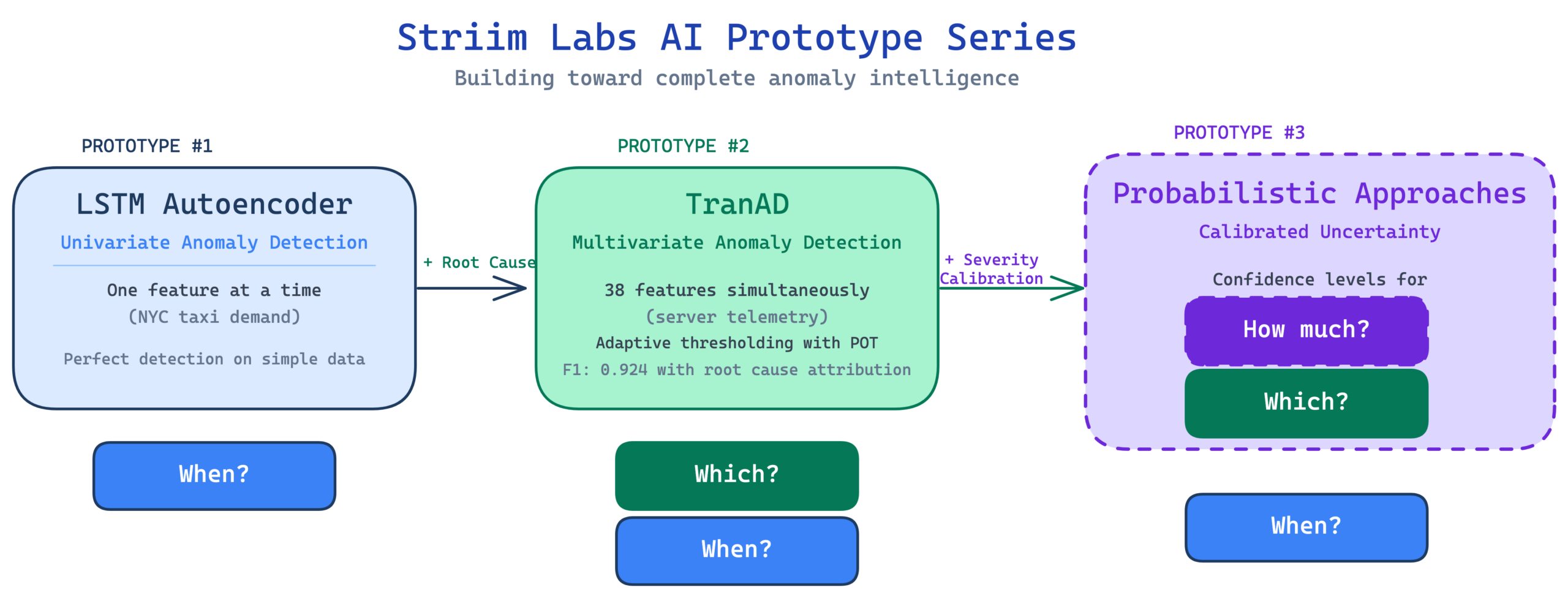
The first prototype identified three limitations of the LSTM autoencoder. It only handles one feature at a time. It can’t tell you how unusual something is. And the threshold doesn’t adapt. This prototype addresses the first gap head on, extending detection from a single time series to 38 features simultaneously. It also adds something the LSTM couldn’t do at all: Root cause attribution tells you not just that something is wrong but which features are causing it.
Why One Feature Isn’t Enough
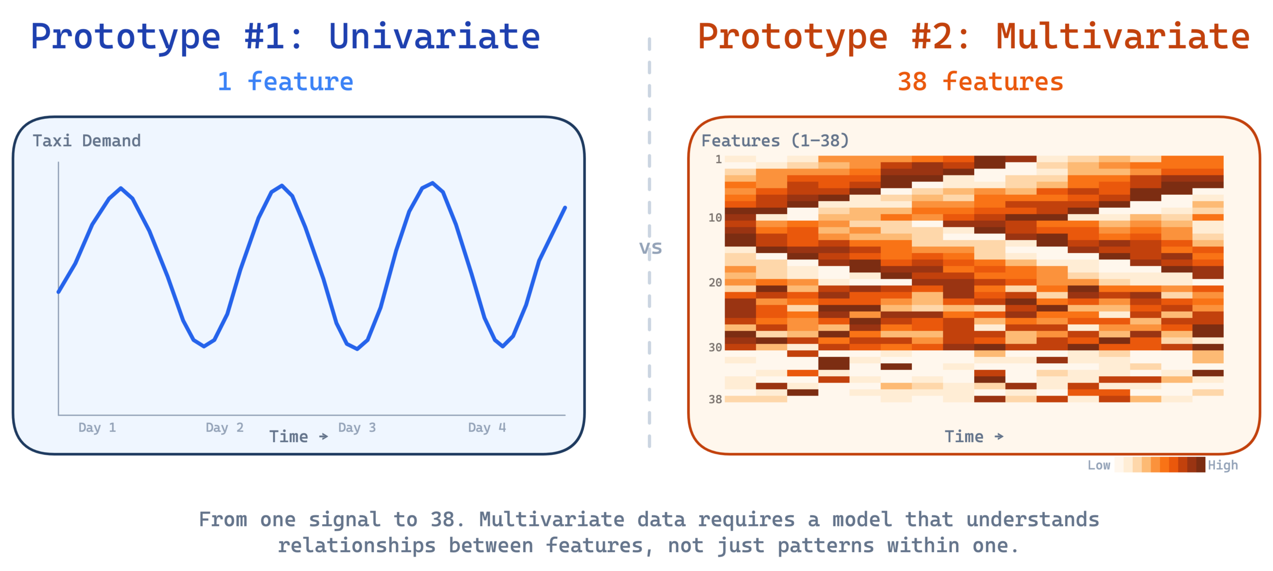
The first prototype monitored a single metric of NYC taxi demand and did it well. But real systems don’t have just one metric. A server has CPU utilization, memory consumption, disk I/O throughput, network traffic, page faults, and dozens more, all moving together in patterns shaped by the workload.
Think of it like a medical checkup. If a doctor only checks your heart rate and sees 95 beats per minute, that’s probably fine. You might have just walked up the stairs. But if your heart rate is 95, your blood pressure is dropping, your temperature is rising, and your oxygen saturation is falling, those four numbers together tell a story that no single number tells on its own. The danger isn’t in any one reading. It’s in the combination.
Server telemetry works the same way. CPU at 90% during a heavy workload is normal. Memory and disk I/O will be high too, and all the numbers make sense together. CPU at 90% when memory is idle, disk is quiet, and network traffic is flat is suspicious. Something is chewing through compute cycles without doing any real work.
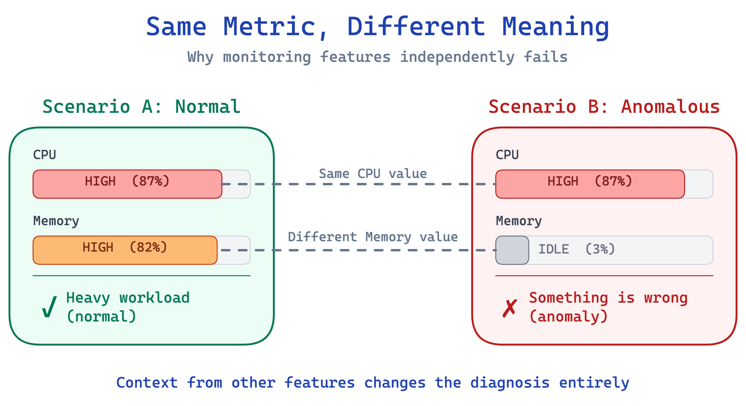
This is why you can’t just run 38 separate univariate detectors and call it a day. The relationships between features carry signal. An anomaly might show up as a subtle shift in how features relate to each other, not as a spike in any single one. A model that looks at each feature in isolation would miss these cross feature patterns entirely.
How TranAD Works
At its core, TranAD is still a reconstruction model. It learns what normal multivariate patterns look like during training and flags deviations at inference time. If the model can reconstruct the input well, the data looks normal. If the reconstruction falls apart, something unusual is happening. This is the same fundamental approach as the LSTM autoencoder from Prototype #1, just applied across all features at once.
But TranAD introduces two innovations that make it far more effective on complex, high dimensional data.
Transformers instead of LSTMs. The LSTM reads a time series step by step, building up context as it goes. A transformer takes a different approach. It looks at all timesteps in the window simultaneously and learns which combinations of features and timesteps matter most for reconstruction.
This is the mechanism known as “attention”. Instead of treating every measurement as equally important, the model learns to focus on the relationships that actually carry signal. For 38 features with complex interactions, this matters. The transformer can learn that a spike in disk writes is only meaningful when paired with specific patterns in memory and network traffic, and weight its reconstruction accordingly.
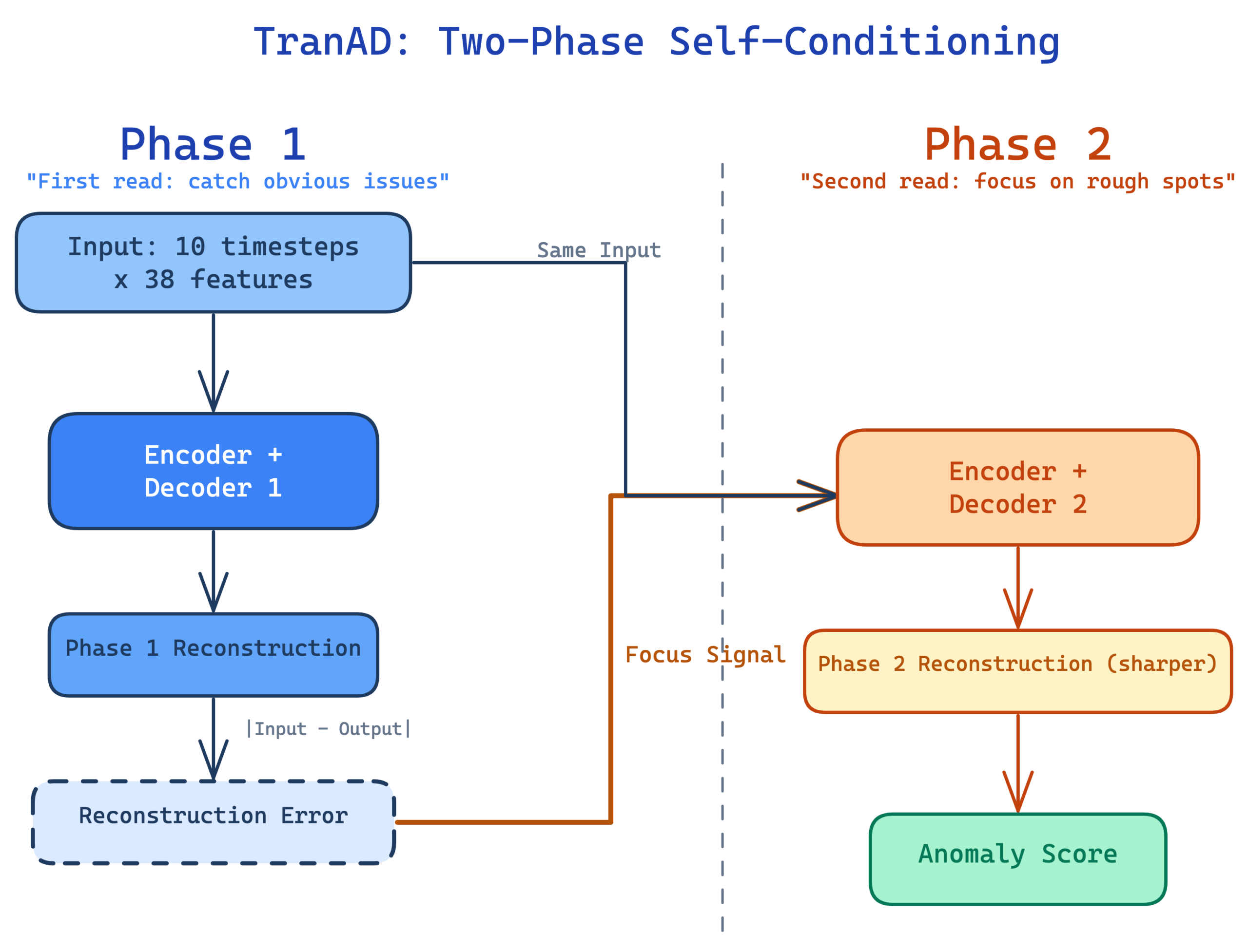
Two phase self conditioning. This is the clever part of the architecture. The model runs its reconstruction twice. Phase 1 produces an initial reconstruction with no prior knowledge of where errors might appear. The model then computes the reconstruction error from Phase 1 and feeds it back as a “focus signal” into Phase 2.
Think of it like proofreading an essay. Your first read catches the obvious issues. Your second read, now that you know where the rough spots are, catches subtler problems because you know exactly where to look. The Phase 2 reconstruction is sharper and produces cleaner separation between normal and anomalous scores.
The original paper also describes an adversarial training objective where the two decoders compete against each other. We explored this during development but found it produced unstable score distributions that broke downstream threshold calibration.
The exponential decay loss weighting from the paper proved far more effective for producing stable, well-separated scores in practice. The idea of this is that early in training, the model is nudged strongly toward accurate reconstruction, and as it stabilizes that pressure gradually fades, letting the model refine the structure of the learned representations without overcorrecting.
The Prototype
Server Machine Dataset
We validated this approach on the Server Machine Dataset (SMD) from the OmniAnomaly project. SMD contains real telemetry from 28 server machines at a large internet company, each recording 38 sensor features (CPU load, memory usage, disk I/O, network metrics) at regular intervals. We trained and evaluated on 4 representative machines.
SMD is the standard benchmark for multivariate anomaly detection. Every major paper in this space, OmniAnomaly, USAD, and TranAD itself, evaluates it. It plays the same role here that the NYC taxi dataset played for the univariate prototype.
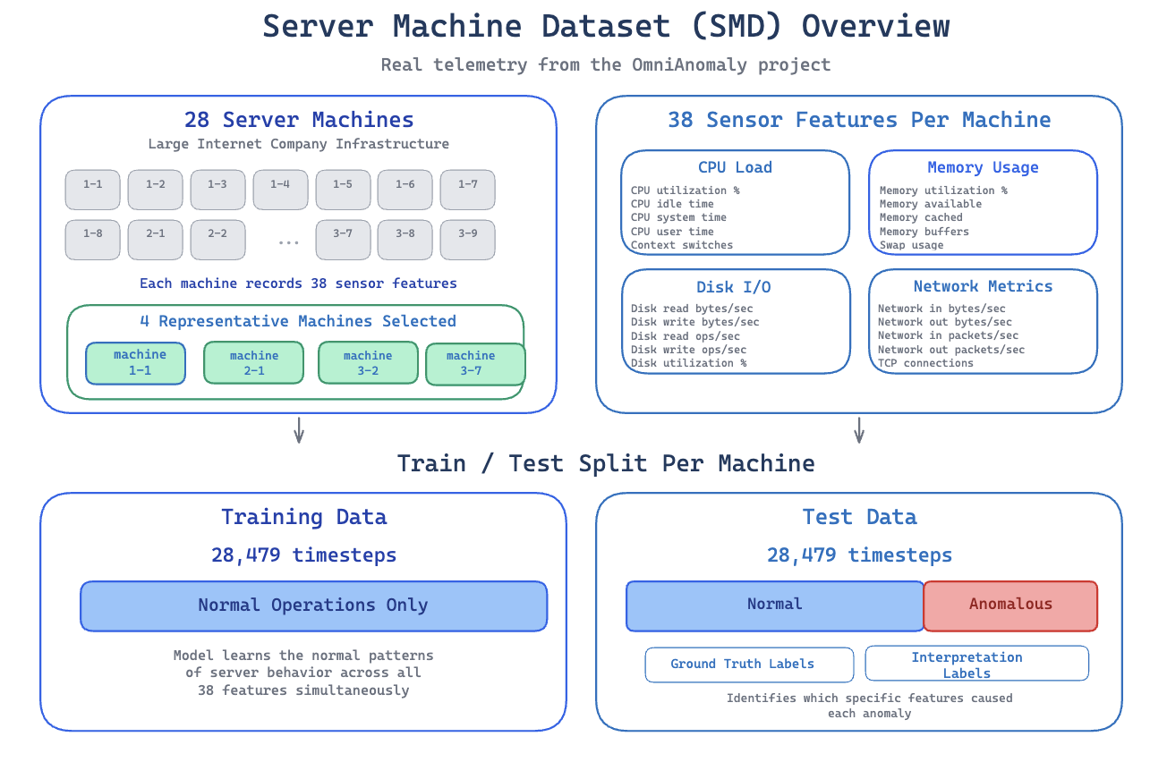
Each machine provides 28,479 timesteps of training data containing normal operations only, and 28,479 timesteps of test data containing both normal and anomalous periods with ground truth labels. The test data also includes interpretation labels identifying which specific features caused each anomaly. This lets us evaluate root cause attribution, not just detection accuracy.
Training
The model processes data in sliding windows of 10 timesteps. Each window captures a short sequence of all 38 features, giving the transformer enough temporal context to learn normal patterns and cross feature relationships.
We used exponential decay loss weighting to control how the training signal shifts between the two reconstruction phases over time. This turned out to be one of the most impactful choices in the entire project. Switching from the paper’s proposed simpler weighting schedule to exponential decay alone improved F1 from 0.795 to 0.921 on our first test machine. The exponential schedule keeps the Phase 1 reconstruction signal strong throughout training, which gives Phase 2 a reliable foundation to build on rather than conditioning on noisy error signals from a first pass that hasn’t converged yet.
Training runs for 20 epochs with a learning rate of 0.0001 using AdamW with gradient clipping. The model has 127,538 parameters, small enough to train on CPU in a few minutes per machine.
Training Data Quality
The first blog post covered the importance of keeping training data clean, since the model learns “normal” from whatever data you give it. TranAD’s two phase architecture provides some natural resilience here. The self conditioning mechanism tends to amplify anomalous patterns rather than absorb them. If a few anomalies slip into the training set, the second pass will see them as high error regions and focus on them.
This actually makes anomalies more likely to be flagged as unusual rather than being quietly learned as normal. It doesn’t eliminate the need for data curation, but it provides an extra layer of safety compared to a standard autoencoder.
Results
Across the 4 reference machines, TranAD achieved an average F1 of 0.924 with strong performance across the board.
<
| Machine | F1 | Precision | Recall | AUC |
| machine-1-1 | 0.926 | 0.862 | 1.000 | 0.992 |
| machine-2-1 | 0.968 | 0.946 | 0.991 | 0.995 |
| machine-3-2 | 0.965 | 0.936 | 0.996 | 0.996 |
| machine-3-7 | 0.835 | 0.718 | 1.000 | 0.981 |
| Average | 0.924 | 0.866 | 0.997 | 0.991 |
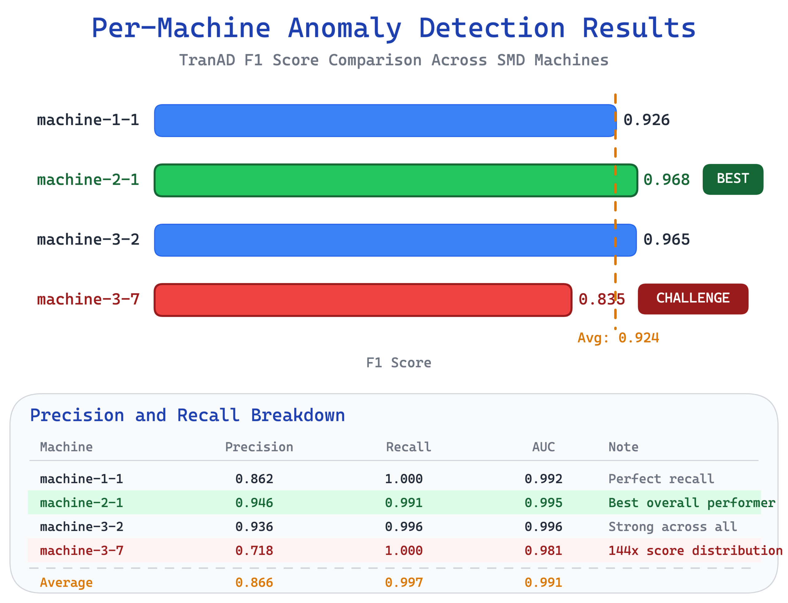
- Machine-2-1 was the standout performer at F1 0.968, with near perfect precision and recall.
- Machine-3-7 was the challenge case at F1 0.835. This machine has an extreme score distribution where test anomaly scores reach 144 times the training average, which makes threshold calibration particularly difficult.
- Two of its five anomaly segments produce scores nearly indistinguishable from normal data, creating a practical ceiling that no amount of threshold tuning could overcome.
For context, the LSTM autoencoder in Prototype #1 achieved perfect detection on its univariate taxi dataset, identifying all 5 known anomalies with zero false positives. That’s impressive, but also a simpler problem. One feature, five clearly distinct anomalies in a strongly periodic signal. TranAD tackles a fundamentally harder problem with 38 features, subtle correlated anomalies across different machines, and still delivers F1 above 0.92 on average.
Root Cause Attribution
This is where TranAD outshines the LSTM prototype. The LSTM could tell you when an anomaly happened, narrowing it down to a 6 hour window within a week. TranAD can tell you when and which features are responsible.
The mechanism is straightforward. The model reconstructs all 38 features independently. When an anomaly is detected, you look at which features have the highest reconstruction error relative to their normal baseline. We call this the elevation ratio. A feature with an elevation ratio of 100 means its reconstruction error is 100 times higher than what the model typically sees during normal operation. Features with high elevation are the ones behaving abnormally.
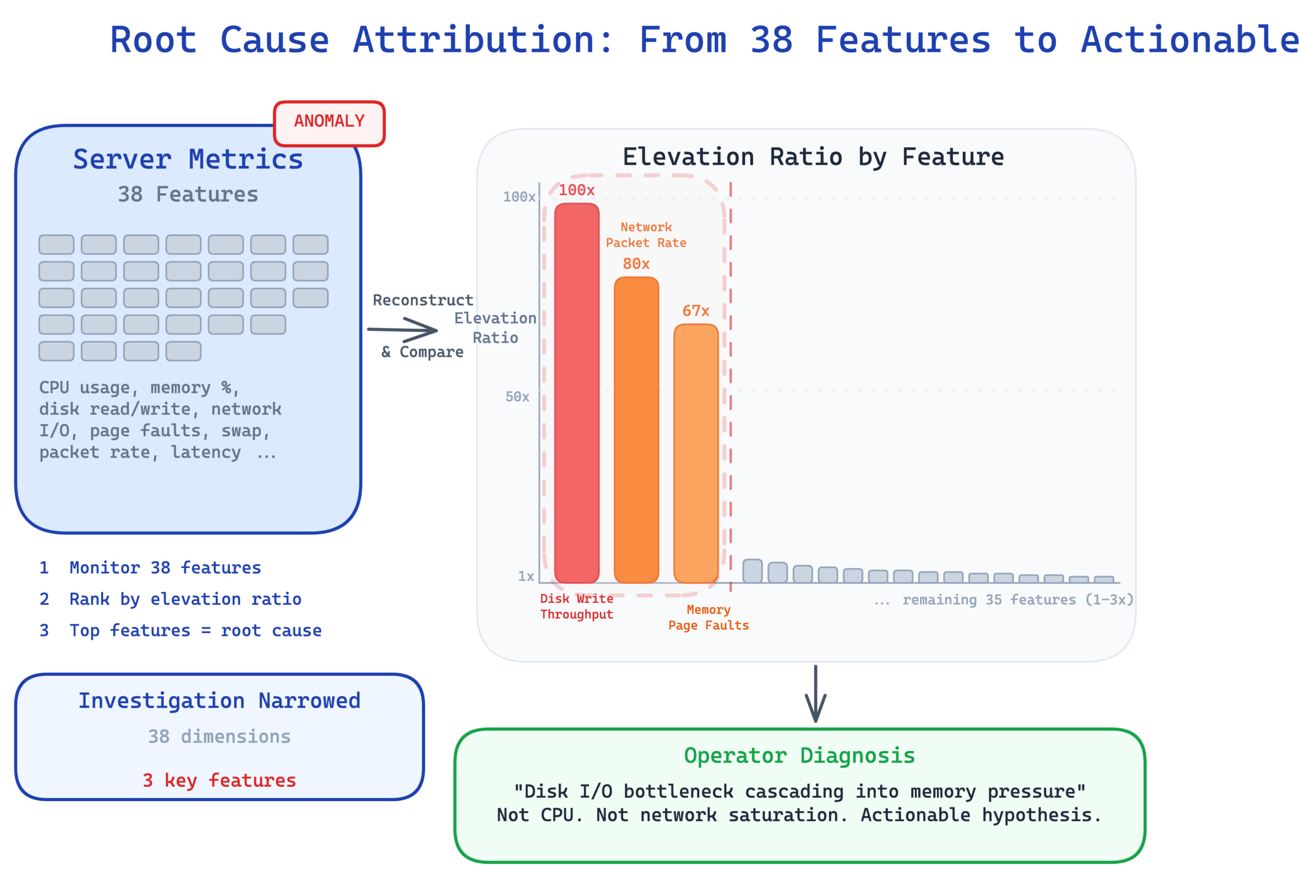
If the model flags a server anomaly and the attribution shows that disk write throughput, network packet rate, and memory page faults have the highest elevation ratios, an operator immediately knows this looks like a disk I/O bottleneck cascading into memory pressure. It’s not a CPU issue. It’s not a network saturation problem. The attribution narrows the investigation from 38 possible dimensions to 2 or 3 and gives the operator a concrete hypothesis to start from.
Attribution quality averaged a HitRate@100% of 0.351 and NDCG@100% of 0.381 across the 4 machines. These metrics measure how well the model’s feature rankings align with the ground truth labels that identify which dimensions actually caused each anomaly. The numbers aren’t perfect, but attribution on multivariate time series is genuinely hard. Even an imperfect ranking that puts the right features in the top 5 out of 38 gives operators a meaningful head start compared to no attribution at all.
Adaptive Thresholding with POT
The first prototype flagged the threshold problem directly. A fixed percentile threshold calibrated on one dataset doesn’t transfer to another. What counts as “unusual” reconstruction error for taxi demand is meaningless for server metrics. Each deployment needs its own calibration.
This prototype addresses that with Peaks Over Threshold (POT), a method from extreme value theory. Instead of picking an arbitrary percentile, POT fits a statistical distribution called the Generalized Pareto Distribution to the tail of the anomaly score distribution. It answers a specific question. Given the pattern of normal scores, how extreme does a new score need to be before it’s statistically implausible? This makes the threshold data driven rather than hand tuned.
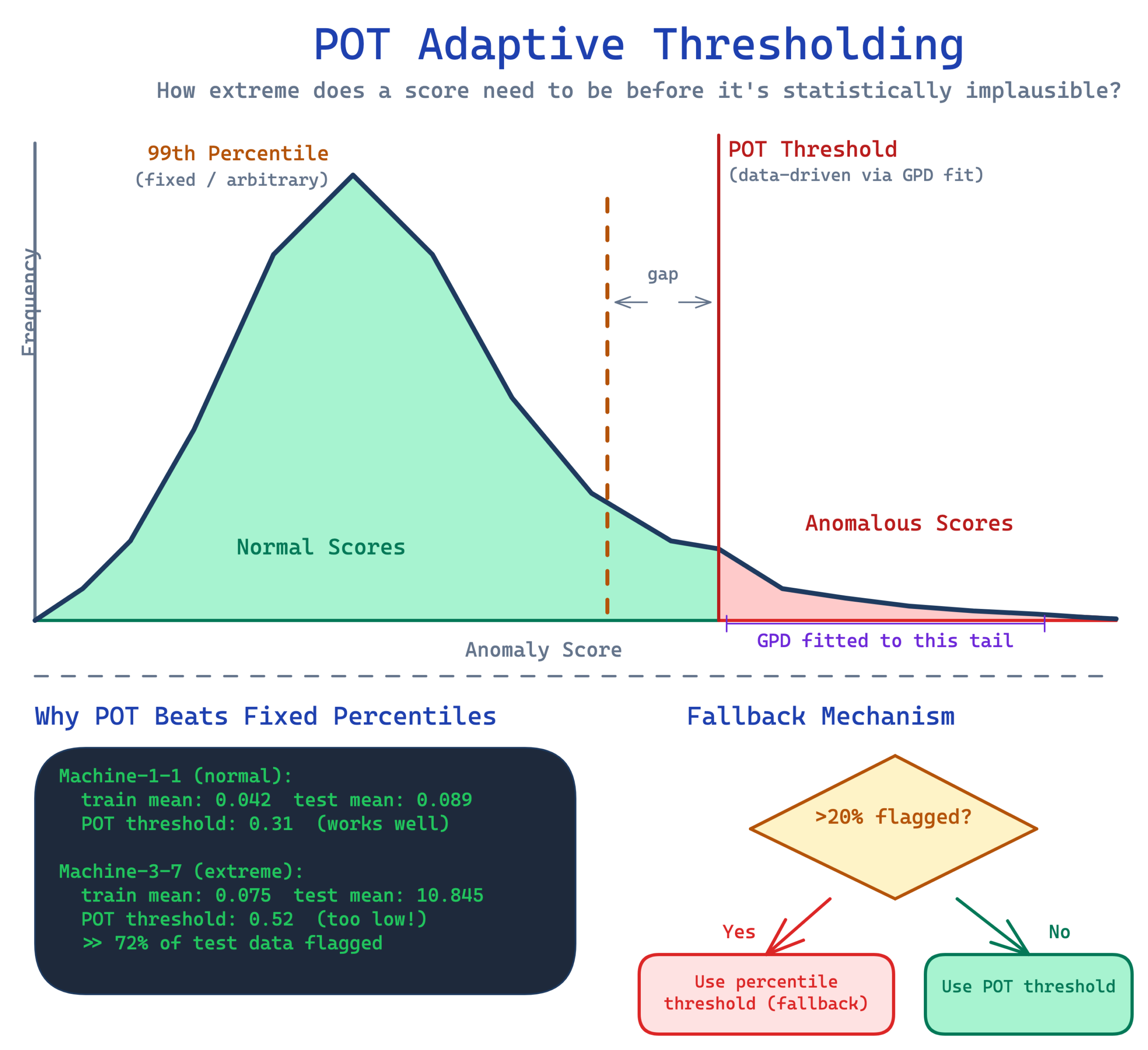
POT worked well on 3 of our 4 machines. Machine-3-7 was the exception. Its extreme score distribution, with a training mean of 0.075 versus a test mean of 10.845, caused POT to set a threshold so low that it flagged nearly all test data as anomalous. We addressed this with a validation step. After computing the POT threshold, the system checks what fraction of data would be flagged. If more than 20% would be classified as anomalous, the system falls back to a conservative percentile threshold instead.
This fallback was essential. It fixed machine-3-7 without regressing the other machines. But it’s worth being honest about the broader picture. Per machine tuning of the POT parameters, specifically the quantile level and scale factor, was still necessary. POT doesn’t eliminate the need for calibration. It makes the calibration more principled and less arbitrary.
From Prototype to Production
The prototype runs as a FastAPI REST API containerized in Docker. Send a batch of raw telemetry data and receive anomaly detection results with per feature root cause attribution. The API handles normalization, windowing, inference, thresholding, and attribution internally. Callers just send raw sensor readings and get structured JSON results back. Inference takes under 20 milliseconds per request on CPU.
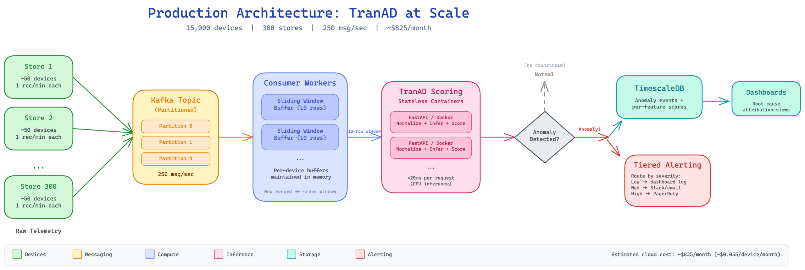
For a production deployment at scale, the architecture extends to handle thousands of devices. Picture 15,000 devices across 300 stores, each pushing one telemetry record per minute. That’s 250 messages per second flowing into a partitioned Kafka topic. Consumer workers maintain per device sliding window buffers of the last 10 records. Every time a new record arrives, the worker scores the full 10 row window against the device’s trained model via the stateless scoring containers. Only anomaly events flow downstream to TimescaleDB for dashboards and to a tiered alerting system that routes based on severity.
The estimated cloud cost for this full deployment is roughly $825 per month, about $0.055 per device per month for real time anomaly detection with sub minute latency and per feature root cause attribution. The key cost insight is that transformer models don’t require GPUs at moderate scale. At 127,000 parameters, CPU inference handles the throughput comfortably.
Beyond the Demo
The model was validated on server telemetry, but the architecture applies to any system where multiple correlated features need simultaneous monitoring. The value proposition goes beyond just detecting anomalies. It’s knowing which features are responsible.
Financial transaction monitoring. Payment processors track dozens of metrics per transaction stream, including volume, average ticket size, decline rates, geographic distribution, and velocity patterns. A fraud ring doesn’t just increase volume. It creates a specific combination of high velocity, unusual geography, and abnormal ticket size that looks very different from a legitimate sales spike. Attribution turns “something is wrong with the East Coast payment stream” into “decline rates and geographic concentration are both abnormal, consistent with card testing.”
Infrastructure and cloud operations. Modern infrastructure generates hundreds of metrics per service, covering latency percentiles, error rates, queue depths, and connection pool utilization. A cascading failure creates a specific fingerprint across these metrics that differs from a simple traffic spike. Root cause attribution can distinguish “the database connection pool is saturated, causing upstream latency” from “traffic increased and everything scaled proportionally.”
Manufacturing and IoT. Industrial equipment with vibration sensors, temperature probes, pressure gauges, and power monitors produces exactly the kind of correlated multivariate data TranAD was designed for. A failing bearing doesn’t just increase vibration. It creates a pattern of rising vibration, rising temperature, and shifting power consumption that the model can detect before any single metric crosses an alarm threshold. Attribution identifies the specific sensor combination, pointing maintenance teams to the right component.
What We Learned
While building this prototype, we learned several practical insights.
- The two phase architecture genuinely helps. This isn’t just a paper trick. The self conditioning mechanism empirically improved score separation between normal and anomalous data. Phase 2 consistently produces sharper, more discriminative scores than Phase 1 alone, because it knows where to focus.
- Loss weighting matters more than you’d expect. The difference between exponential decay and epoch inverse weighting was the single largest factor in our F1 improvement, bigger than learning rate tuning, architecture variants, or scoring mode selection. The weighting controls how quickly training shifts emphasis to the self conditioned phase, and getting this wrong degrades everything downstream.
- Root cause attribution is valuable even when imperfect. Operators don’t need a perfect feature ranking. They need a starting point. Going from “something is wrong with server 7” to “disk writes and memory page faults are abnormal” saves real investigation time, even if the model occasionally misranks the third or fourth most important feature.
- POT thresholding is powerful but not magic. Extreme value theory gives you a principled framework for setting thresholds, and that’s a real improvement over arbitrary percentiles. But per machine calibration was still necessary, and extreme score distributions can break the method entirely. The fallback mechanism is not optional.
- Transformers on CPU are viable at scale. The model runs inference in under 20 milliseconds on CPU. At 127,000 parameters, there’s no need for GPU infrastructure at moderate device counts. This keeps deployment costs low and infrastructure simple.
Where This Model Hits Its Limits
After spending real time with this model, here’s where I think it actually breaks down.
- The 10 timestep window is more restrictive than it sounds. It works well for anomalies that manifest within minutes to tens of minutes, which covers a lot of real workloads. But anything with slow onset (gradual memory leaks over days, seasonal drift over weeks) just won’t land in that window. The model sees each window independently and has no mechanism for tracking gradual change across successive windows. You could widen the window, but you pay for it in compute and in dilution of the cross feature signal that makes TranAD work in the first place.
- Attribution is the feature I’m most excited about…and also the one that gives me pause. When it works, it’s genuinely useful. Going from “machine-2-1 is anomalous” to “disk I/O and memory paging are abnormal” is a real win for an operator. But the quality varies a lot. Machine-3-2 hit detection F1 of 0.965 and near zero on attribution, because the dimensions actually driving the anomaly didn’t align with where the model placed its reconstruction error. You get the detection but the explanation collapses. Attribution lands best when a small number of features drive the anomaly. When the anomaly is spread across many dimensions, the feature ranking starts to look like noise.
- The stationarity assumption is the elephant in the room. The model assumes “normal” doesn’t move. In any production system worth monitoring, “normal” moves constantly: new deployments, capacity upgrades, workload mix changes, all of it shifts the baseline. There’s nothing in this architecture that detects when the model’s definition of normal has gone stale, and nothing that retrains it when that happens. That’s the gap I find most important, and it’s exactly the one I’m targeting next.
Overall, my impression is that TranAD is a strong fit when you have a high dimensional system, short horizon anomalies, and a small number of features tend to drive each anomaly. Server telemetry is basically the canonical example, which is why the SMD numbers look as good as they do. It’s a weaker fit when anomalies are slow, distributed across many dimensions, or when the underlying system is non-stationary in ways that move faster than your retraining cadence.
The transformer plus self conditioning is a real architectural step forward, but it’s not a free lunch, and I’d rather be upfront about where the cracks are than oversell it.
What’s Next
The first prototype handled one feature at a time. This second prototype handles 38 features at once and tells you which ones are responsible. But one limitation from the original LSTM blog remains unaddressed. Neither model can tell you how unusual something is. They produce anomaly scores that cross a threshold, but those scores aren’t calibrated probabilities. The model can’t distinguish a 1 in 10,000 event from a 1 in 1,000,000 event.
The next prototype will tackle that gap with probabilistic approaches that produce calibrated uncertainty estimates, giving you not just “is this anomalous” but “how anomalous” with a meaningful confidence level.
Each prototype in this series builds on the last, working toward a comprehensive anomaly detection toolkit that matches the right technique to the right problem.