This is the first AI Prototype in our anomaly detection series from Striim Labs. We start with the LSTM autoencoder, a model that learns the rhythm of your data and flags anything that doesn’t fit.
Ready to dive in with LSTM? Click here to jump into the Github repo and test the prototype for yourself!
Got questions? Reach out to us at striimlabs@striim.com
Detecting Anomalies in Streaming Time Series Data
As we announced recently, we’re excited to introduce Striim Labs: an applied research group focused on delivering working “AI Prototypes” at the intersection of AI/ML and real-time data streaming. To kick things off, we’ll be sharing a prototype model LSTM autoencoder, the first in our series on anomaly detection.
The prototype is based on the EncDec-AD architecture from Malhotra et al. (2016), “LSTM-based Encoder-Decoder for Multi-Sensor Anomaly Detection.” This paper was one of the first to show that an LSTM encoder-decoder trained only on normal data could reliably detect anomalies through reconstruction error alone. To this day it remains the baseline that nearly every new anomaly detection paper benchmarks against.
We chose it as our starting point for the same reason, it’s the most intuitive approach, it performs well on data with strong periodic patterns, and it gives us a clear foundation to build on as the series progresses into more sophisticated techniques.
Let’s dig into the model, the problem it solves, and the AI Prototype you can deploy in your own environment.
The Problem: Finding Needles in a Haystack of Data
Every business generates streams of data such as transaction volumes, server metrics, customer activity, sensor readings. Most of the time, the data follows predictable patterns, such as when retail spend spikes during the holidays and taxi demand surges at rush hour.
But occasionally, something unexpected happens, whether an unexpected weather event or an unforeseen incident. These events are rare, unpredictable, and often costly.
Traditional rule based systems require you to define what “abnormal” means upfront, such as “flag any transaction over $10,000” or “alert if CPU exceeds 90% usage”. But the most dangerous anomalies are the ones you haven’t thought of yet.
What if, instead of defining every possible anomaly, we could teach a model what “normal” looks like, and simply let it flag anything else?
That’s exactly what an LSTM autoencoder does.
Why LSTM?
The “LSTM” in the name stands for Long Short-Term Memory, a type of neural network that can remember context over long sequences. This matters because a single data point means very different things depending on when it occurs.
At 3 AM, 5,000 passengers is high. Something unusual might be happening.
At 5 PM, 5,000 passengers is low. Rush hour should be much busier.
A simple model that looks at each data point in isolation would miss this context. The LSTM reads the entire sequence and understands the position of each value within the broader pattern. It knows what Monday morning looks like versus Saturday night, and it knows when a value is normal for its time slot versus when it’s an outlier.
The Copycat Test
The core idea behind an autoencoder is surprisingly intuitive. Think of it like a game of telephone.
You play a song for someone (feed data into the model)
They listen and try to memorize it (the model compresses the data)
They hum it back to you (the model reconstructs the data)
If the song is one they’ve heard hundreds of times, they’ll hum it back almost perfectly. But if you play something completely unfamiliar, their attempt to hum it back will sound off. The gap between the original and their reproduction tells you how “unusual” the input was. That gap is called the reconstruction error, and it’s the heart of anomaly detection with autoencoders. High error means the model is struggling to reproduce the input, which means the input doesn’t match the patterns it learned during training.
The key insight is that we only train the model on normal data. It never sees anomalies during training. So when an anomaly appears, the model has no idea how to reproduce it, and the reconstruction error spikes. This is what makes the approach powerful as we don’t need labeled examples of every possible anomaly. We just need enough normal data to teach the model what “normal” looks like.
That gap is called the reconstruction error, and it’s the heart of anomaly detection with autoencoders. High error means the model is struggling to reproduce the input, which means the input doesn’t match the patterns it learned during training.
The key insight is that we only train the model on normal data. It never sees anomalies during training. So when an anomaly appears, the model has no idea how to reproduce it, and the reconstruction error spikes. This is what makes the approach powerful as we don’t need labeled examples of every possible anomaly. We just need enough normal data to teach the model what “normal” looks like.
Architecture designed for sequential data
The model we built is called a Long Short-Term Memory Autoencoder (LSTM-AE), a neural network architecture specifically designed for sequential data like time series. Here’s how the pieces fit together.
The Bottleneck
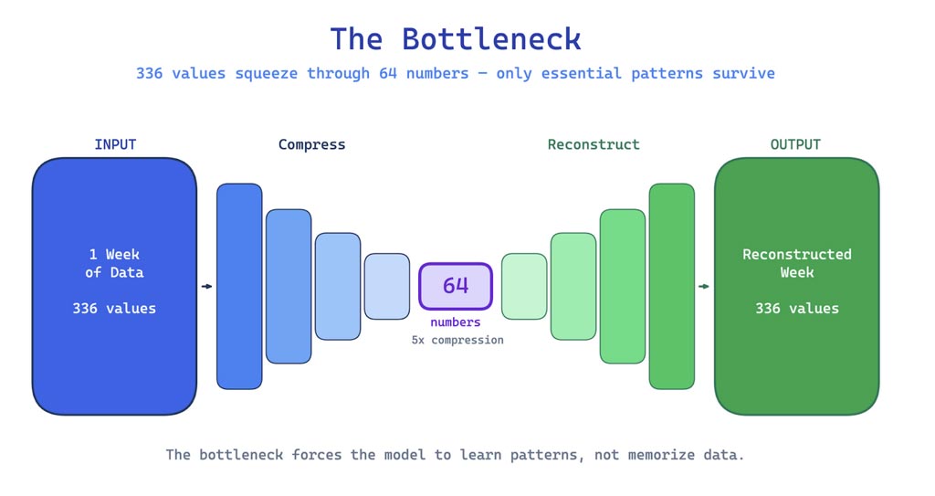
The architecture has an hourglass shape. Data flows in wide, gets squeezed through a narrow bottleneck, and then gets expanded back out.
Input is one full week of data, 336 measurements taken every 30 minutes (48 per day x 7 days)
Bottleneck is where the model compresses that entire week down to just 64 numbers
Output is the model’s reconstruction of the full 336 measurement week from those 64 numbers
That’s a 5x compression ratio. The model can’t memorize every data point, it’s forced to learn the underlying pattern instead. This is also key as learning every data point is both impracticable and leads to poor generalization.
We found that compression is what makes the model useful for anomaly detection. When the input follows the normal pattern the model has learned (daily rush hour peaks, nightly lulls, weekend dips), it can compress and reconstruct it faithfully. But when the input contains something the model hasn’t seen, like a sudden spike or an unusual drop, the bottleneck can’t capture it and the reconstruction falls apart.
The Prototype: Testing on NYC Taxi Passenger Data
To validate this approach, we built a working prototype using a well known benchmark dataset, NYC taxi passenger demand from July 2014 through January 2015. The dataset contains roughly 10,000 measurements taken every 30 minutes, or about 29 complete weeks of data.
Why Taxi Data?
NYC taxi demand is ideal for prototyping because it has strong, repeating patterns that are easy to understand.
Daily cycles where demand peaks during morning and evening rush hours, then drops overnight
Weekly cycles where weekdays are busier than weekends
Predictable rhythms where the pattern repeats week after week with minor variations
More importantly, the dataset contains 5 known real world anomalies that disrupted the normal pattern in ways that are easy to verify.
Event
What Happened
Impact
NYC Marathon (Nov 2, 2014)
Massive citywide event
Demand spiked ~50% above normal
Thanksgiving (Nov 27, 2014)
National holiday
Extended demand drop
Christmas (Dec 25, 2014)
National holiday
Demand dropped to about 2,000 passengers (92% below normal)
New Year’s (Dec 31, 2014)
Holiday celebration
Multi-day demand disruption
January Blizzard (Jan 26, 2015)
Major winter storm
Citywide transportation shutdown
Training on Normal Weeks Only
We split the 29 weeks of data carefully.
8 normal weeks for training so the model only sees regular patterns
6 normal weeks for validation and threshold calibration
15 weeks for testing containing a mix of normal weeks and all 5 anomaly weeks
The model trains by trying to reconstruct each normal week as accurately as possible. Over about 100 training cycles (epochs), it gradually learns the daily and weekly rhythms of NYC taxi demand. Training stops automatically when the model’s accuracy plateaus, a technique called early stopping.
After training, we measure how well the model reconstructs the validation data and set a detection threshold at the 99.99th percentile of reconstruction errors on normal data. Anything above that threshold is flagged as anomalous.
How to Keep Training Data Clean
Since the model learns “normal” from its training data, the quality of that training data matters. In our taxi dataset the anomalies are well documented, so we know exactly which weeks to exclude. But in a real world deployment, how do you guarantee your training data doesn’t contain unlabeled anomalies that could silently corrupt what the model learns as “normal”?
The most practical approach is to work with subject matter experts to curate a training window. Select a time period that domain experts are confident represents normal operations. For most operational data this is straightforward, just pick two months where nothing unusual happened. A smaller, vetted dataset is far more valuable than a large one that might be contaminated.
The LSTM autoencoder itself doesn’t have built in resilience to training data contamination, which is one reason it works best as a starting point with carefully curated data. Later prototypes in this series incorporate modified training objectives that automatically down weight suspicious points during training, so even if a few anomalies slip into the training set, they don’t corrupt the learned model. We’ll cover those techniques in detail when we get to them.
Results:
On the test set, the model correctly identified all 5 anomaly weeks without a single false positive.
But raw detection isn’t the whole story. The system also localizes anomalies within each week, narrowing down the alert from “this week is unusual” to “the anomaly is in this specific 6 hour window.” This is critical for operational use because an operator investigating an alert needs to know when to look, not just that something happened somewhere in a 7 day span.
Christmas Day (demand drop). The model expected typical weekday demand patterns. When Christmas demand plummeted, the model’s reconstruction showed what a normal day should look like, making the gap enormous. It’s also worth noting that the entire Christmas week shows slightly lower demand overall, but the model didn’t flag every point in the window. It was able to distinguish between “a little quieter than usual” and “something is genuinely wrong,” zeroing in on the actual collapse in demand rather than the surrounding dip. A simple rule based approach that just checks whether values fall below a fixed threshold would have either missed the real anomaly or flagged the entire week indiscriminately.
In every case, the detection logic is the same. The model tries to “copy” the week, fails at the unusual parts, and the gap between original and copy reveals exactly where and how the anomaly occurred.
From Prototype to Production
During the course of this research, we discovered that a model that works on historical data is useful for research, but a model that works in real time is useful for operations. With that in mind, we built a full streaming pipeline to prove the approach works end to end.
The Architecture
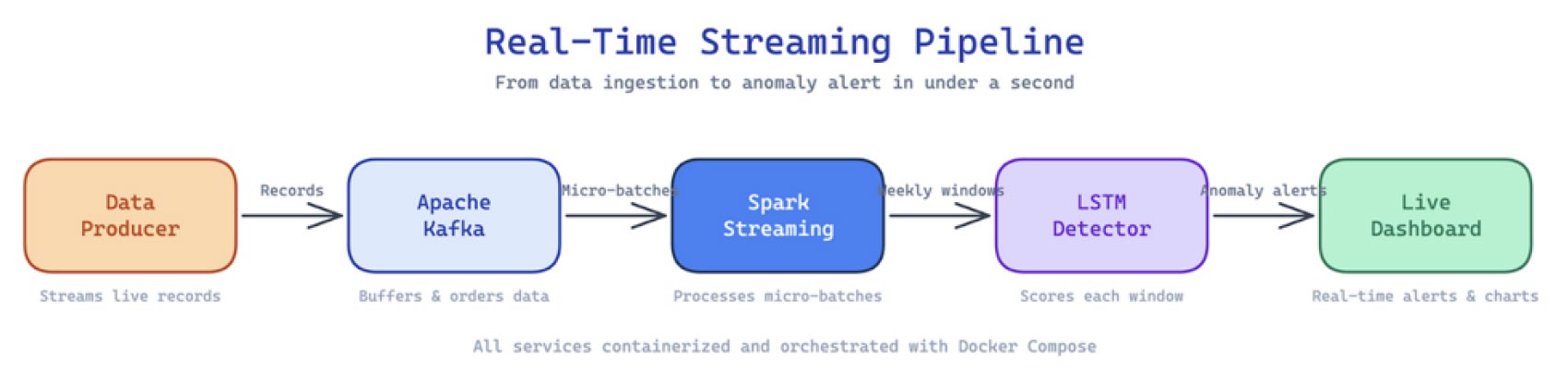
The system runs as a set of containerized services orchestrated with Docker.
Data Producer streams records into Apache Kafka, simulating a live data feed
Apache Kafka acts as the message queue, buffering incoming data
Apache Spark (Structured Streaming) consumes data from Kafka in micro batches
LSTM Detector processes each complete week of data through the trained model
Dash Dashboard displays results in real time, showing incoming data, detected anomalies, and the localized 6 hour windows where anomalies occurred
The entire pipeline runs with docker compose up, streaming from the first data point to anomaly alert on a live dashboard. When the model detects an anomaly, the dashboard highlights the specific time window in red, showing operators exactly when and where the disruption occurred.
Beyond the Demo
NYC taxi data makes a great demo, but the model doesn’t know anything about taxis. It learned a pattern in the repeating weekly rhythm with daily subcycles. That same pattern exists in virtually any operational data.
Financial transaction monitoring. Payment processors see predictable daily and weekly volume patterns, higher during business hours, lower overnight, minimal on weekends. A flash crash, fraud ring activation, or system outage disrupts that rhythm in exactly the same way a marathon or blizzard disrupts taxi demand.
Infrastructure monitoring. Server CPU, memory, and network traffic follow daily usage patterns. An outage, DDoS attack, or misconfigured deployment creates the same kind of spike or drop that the model is designed to catch.
IoT and manufacturing. Sensor readings from industrial equipment follow operating cycles. A failing bearing, overheating motor, or process deviation breaks the expected pattern.
The model doesn’t need to be retrained from scratch for each domain. The architecture itself is domain agnostic. You feed it normal data from your domain, it learns your patterns, and it flags deviations from your normal.
What We Learned
Building this prototype surfaced several practical insights.
Training on normal data only is powerful and practical. In most real world scenarios, labeled anomaly data is scarce or nonexistent. This approach only requires a representative sample of normal behavior, which is almost always available.
The bottleneck is doing the heavy lifting. The 5x compression ratio (336 values to 64 numbers) is what forces the model to learn patterns rather than memorize data. Too much capacity and the model memorizes everything, including anomalies. Too little and it can’t reconstruct normal data accurately enough. The 64 unit hidden dimension hit the sweet spot for this dataset.
Localization matters as much as detection. Knowing that “this week is anomalous” is a starting point. Knowing that “the anomaly is concentrated in this 6 hour window on Tuesday afternoon” is actionable. The sliding window localization technique adds significant operational value with minimal additional computation.
Streaming is where the value lives. The model achieves sub second inference per weekly window. Combined with the Kafka and Spark pipeline, this means anomalies can be surfaced within seconds of the data arriving, fast enough for real time operational response.
Failure to Adapt: Where This Model Hits Its Limits
The LSTM autoencoder performed flawlessly on our taxi dataset, but the approach has inherent tradeoffs worth understanding. These limitations also motivate the alternative prototypes we explore later in this series.
It needs data with a strong repeating cycle. The model learns a dominant periodic pattern (in our case, a weekly rhythm with daily subcycles) and flags deviations from it. If your data has no clear periodicity, or the dominant cycle is shorter than about 50 time steps, reconstruction based detection adds complexity without much benefit. Simpler methods like Isolation Forest tend to outperform in those scenarios.
It can tell you something is unusual, but not how unusual. Reconstruction error measures whether data “looks different” from normal, but it doesn’t model a probability distribution. The model can’t distinguish a 1 in 10,000 event from a 1 in 1,000,000 event. For use cases like financial risk scoring that need calibrated anomaly likelihoods, probabilistic models like variational autoencoders are better suited.
The threshold doesn’t adapt over time. Our detection threshold is a fixed percentile set from a single validation set. That threshold won’t transfer to a new domain because what’s “normal” reconstruction error for taxi demand is meaningless for financial transactions or server metrics. Each deployment requires its own calibration and testing to avoid being too sensitive (false alarms) or too lenient (missed anomalies). Adaptive approaches like Peaks Over Threshold (POT) can reduce this burden, and later prototypes in this series incorporate that flexibility.
What’s Next
This LSTM autoencoder is the first AI Prototype in our anomaly detection series. It excels at learning normal behavior from unlabeled data with strong temporal patterns, but as the limitations above reveal, no single model covers every scenario. In upcoming prototypes, we’ll tackle those gaps head on.
Probabilistic scoring with variational autoencoders that can quantify how unlikely an observation is, not just flag that it’s different
Multivariate modeling where the relationships between features matter as much as temporal patterns
Adaptive thresholding with approaches that adjust to non stationary data, so detection stays calibrated even as “normal” evolves
Each AI Prototype in the series builds on the lessons of the previous one, working toward a comprehensive anomaly detection toolkit that matches the right approach to the right data.
Try It Yourself
The full prototype is open source and ready to deploy, try it yourself here.
We built this prototype to start a conversation, not end one. If you’re working on anomaly detection in your own domain, we’d love to hear what’s working, what isn’t, and what you’d like to see from a real-time detection prototype.
Drop us a line at striimlabs@striim.com or connect with us on LinkedIn.
This is just the first prototype in the series. Follow us on Medium to get notified when we publish the next one: TranAD, a transformer-based model that monitors dozens of features at once and tells you which ones are causing trouble..

 That gap is called the reconstruction error, and it’s the heart of anomaly detection with autoencoders. High error means the model is struggling to reproduce the input, which means the input doesn’t match the patterns it learned during training.
The key insight is that we only train the model on normal data. It never sees anomalies during training. So when an anomaly appears, the model has no idea how to reproduce it, and the reconstruction error spikes. This is what makes the approach powerful as we don’t need labeled examples of every possible anomaly. We just need enough normal data to teach the model what “normal” looks like.
That gap is called the reconstruction error, and it’s the heart of anomaly detection with autoencoders. High error means the model is struggling to reproduce the input, which means the input doesn’t match the patterns it learned during training.
The key insight is that we only train the model on normal data. It never sees anomalies during training. So when an anomaly appears, the model has no idea how to reproduce it, and the reconstruction error spikes. This is what makes the approach powerful as we don’t need labeled examples of every possible anomaly. We just need enough normal data to teach the model what “normal” looks like.

 In every case, the detection logic is the same. The model tries to “copy” the week, fails at the unusual parts, and the gap between original and copy reveals exactly where and how the anomaly occurred.


 That gap is called the reconstruction error, and it’s the heart of anomaly detection with autoencoders. High error means the model is struggling to reproduce the input, which means the input doesn’t match the patterns it learned during training.
The key insight is that we only train the model on normal data. It never sees anomalies during training. So when an anomaly appears, the model has no idea how to reproduce it, and the reconstruction error spikes. This is what makes the approach powerful as we don’t need labeled examples of every possible anomaly. We just need enough normal data to teach the model what “normal” looks like.
That gap is called the reconstruction error, and it’s the heart of anomaly detection with autoencoders. High error means the model is struggling to reproduce the input, which means the input doesn’t match the patterns it learned during training.
The key insight is that we only train the model on normal data. It never sees anomalies during training. So when an anomaly appears, the model has no idea how to reproduce it, and the reconstruction error spikes. This is what makes the approach powerful as we don’t need labeled examples of every possible anomaly. We just need enough normal data to teach the model what “normal” looks like.
 In every case, the detection logic is the same. The model tries to “copy” the week, fails at the unusual parts, and the gap between original and copy reveals exactly where and how the anomaly occurred.