In this series of blog-based tutorials, we are guiding you through the process of building data flows for streaming integration and analytics applications using the Striim platform. This tutorial focuses on SQL-based stream processing for Apache Kafka with in-memory enrichment of streaming data. For context, please check out Part One of the series where we created a data flow to continuously collect change data from MySQL and deliver as JSON to Apache Kafka.
In this tutorial, we are going to process and enrich data-in-motion using continuous queries written in Striim’s SQL-based stream processing language. Using a SQL-based language is intuitive for data processing tasks, and most common SQL constructs can be utilized in a streaming environment. The main differences between using SQL for stream processing, and its more traditional use as a database query language, are that all processing is in-memory, and data is processed continuously, such that every event on an input data stream to a query can result in an output.
The first thing we are going to do with the data is extract fields we are interested in, and turn the hierarchical input data into something we can work with more easily.
Transforming Streaming Data With SQL
You may recall the data we saw in part one looked like this:
| data | before | metadata |
|---|---|---|
[86,466,869,1522184531000]</code> |
[86,466,918,1522183459000]</code> |
{ |
This is the structure of our generic CDC streams. Since a single stream can contain data from multiple tables, the column values are presented as arrays which can vary in size. Information regarding the data is contained in the metadata, including the table name and operation type.
The PRODUCT_INV table in MySQL has the following structure:
LOCATION_ID int(11) PK
PRODUCT_ID int(11) PK
STOCK int(11)
LAST_UPDATED timestamp
The first step in our processing is to extract the data we want. In this case, we only want updates, and we’re going to include both the before and after images of the update for stock values.
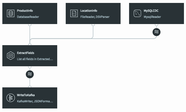
To do the processing, we need to add a continuous query (CQ) into our dataflow. This can be achieved in a number of ways in the UI, but we will click on the datastream, then on the plus (+) button, and select “Connect next CQ component” from the menu.
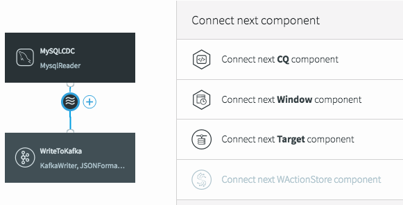
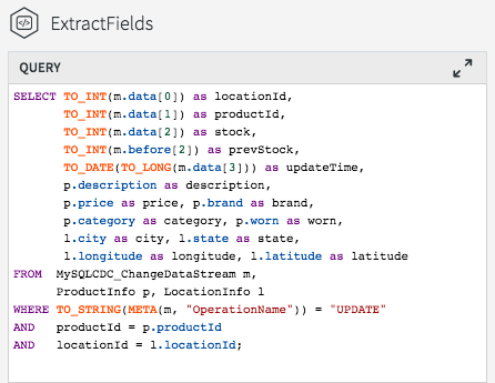
As with all components in Striim, we need to give the CQ a name, so let’s call it “ExtractFields”. The processing query defaults to selecting everything from the stream we were working with.
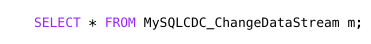
But we want only certain data, and to restrict things to updates. When selecting the data we want, we can apply transformations to convert data types, access metadata, and many other data manipulation functions. This is the query we will use to process the incoming data stream:
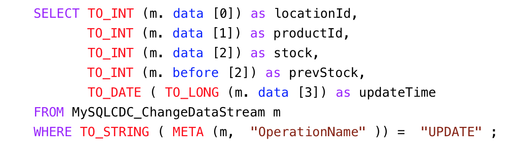
Notice the use of the data array (what the data looks like after the update) in most of the selected values, but the use of the before array to obtain the prevStock.
We are also using the metadata extraction function (META) to obtain the operation name from the metadata section of the stream, and a number of type conversion functions (TO_INT for example) to force data to be of the correct data types. The date is actually being converted from a LONG timestamp representing milliseconds since the EPOCH.
</code>
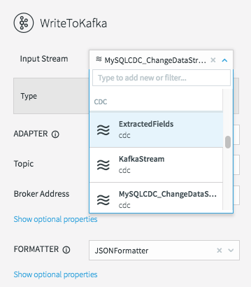
The final step before we can save this CQ is to choose an output stream. In this case we want a new stream, so we’ll call it “ExtractedFields”.
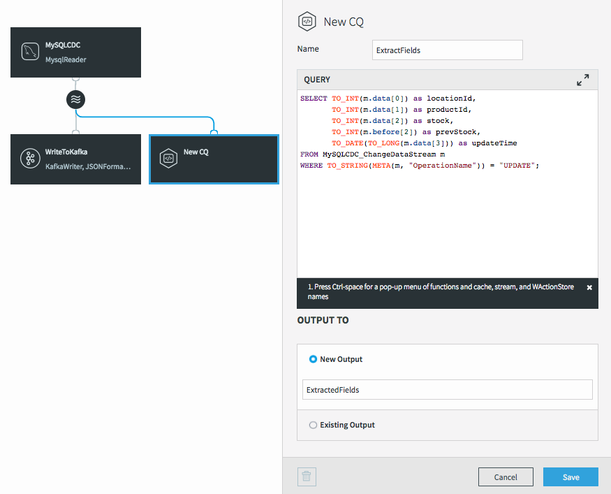
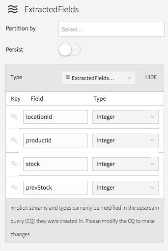
When we click on Save, the query is created alongside the new output stream, which has a data type to match the projections (the transformed data we selected in the query).
The data type of the stream can be viewed by clicking on the stream icon.
There are many different things you can do with streams themselves, such as partition them over a cluster, or switch them to being persistent (which utilizes our built-in Apache Kafka), but that is a subject for a later blog.
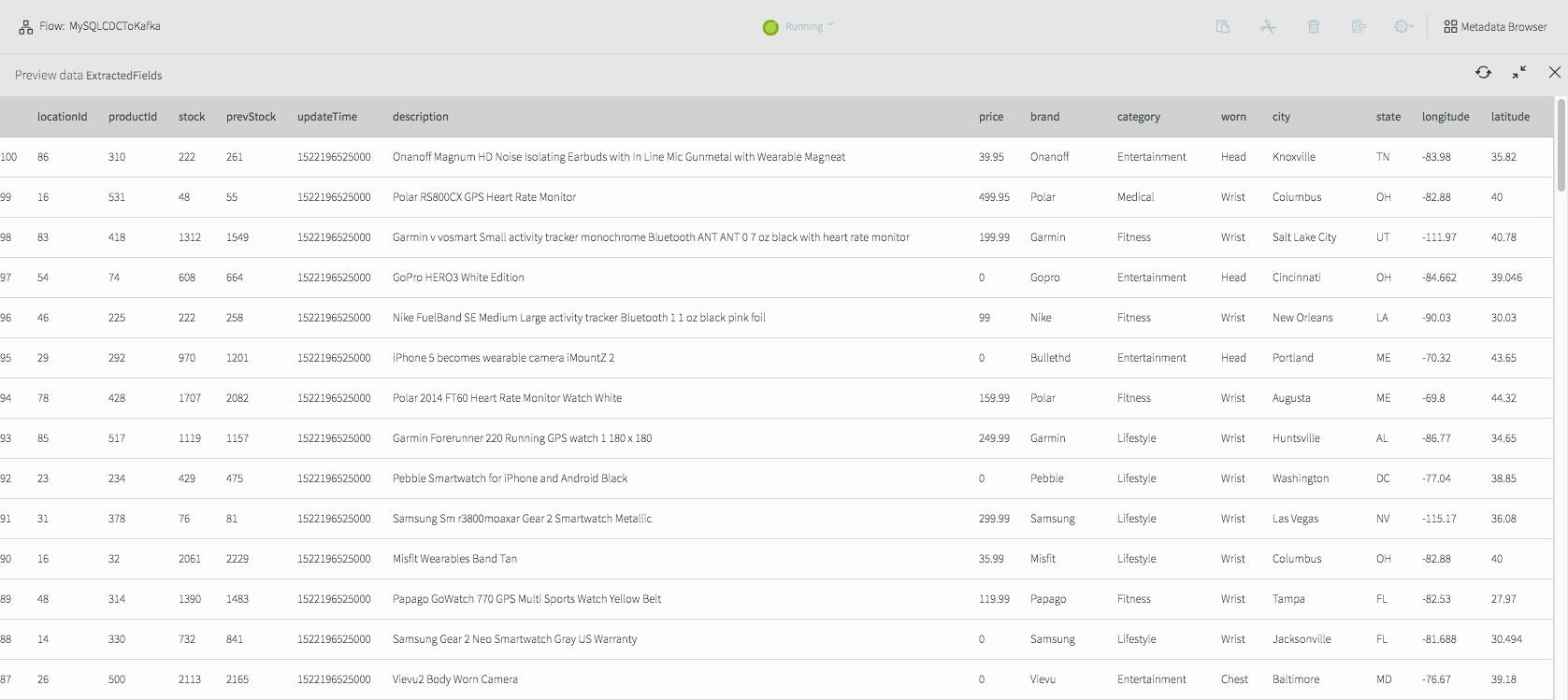
If we deploy and start the application (see the previous blog for a refresher) then we can see what the data now looks like in the stream.
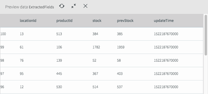
As you can see it looks very different from the previous view and now only contains the fields we are interested in for the remainder of the application.
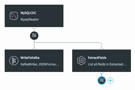
But at the moment, this new stream currently goes nowhere, while the original data is still being written to Kafka.
Writing Transformed Data to Kafka
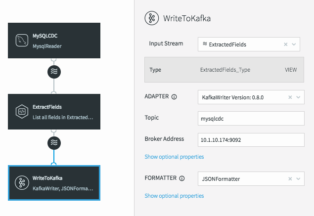
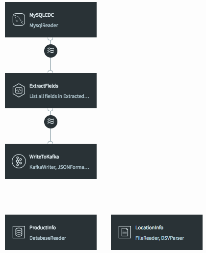
To fix this, all we need to do is change the input stream for the WriteToKafka component.
This changes the data flow, making it a continuous linear pipeline, and ensures our new simpler data structure is what is written to Kafka.
Utilizing Caches For Enrichment
Now that we have the data in a format we want, we can start to enrich it. Since the Striim platform is a high-speed, low latency, SQL-based stream processing platform, reference data also needs to be loaded into memory so that it can be joined with the streaming data without slowing things down. This is achieved through the use of the Cache component. Within the Striim platform, caches are backed by a distributed in-memory data grid that can contain millions of reference items distributed around a Striim cluster. Caches can be loaded from database queries, Hadoop, or files, and maintain data in-memory so that joining with them can be very fast.
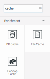
In this example we are going to use two caches – one for product information loaded from a database, and another for location information loaded from a file.

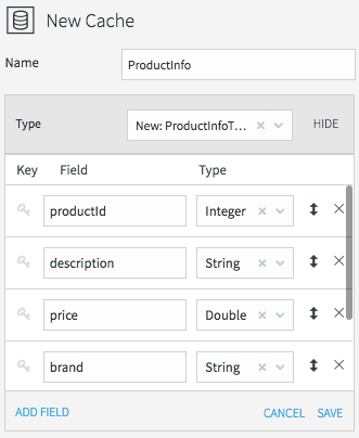
All caches need a name, data type, lookup key, and can optionally be refreshed periodically. We’ll call the product information cache “ProductInfo,” and create a data type to match the MySQL PRODUCT table, which contains details of each product in our CDC stream. This is define in MySQL as:
PRODUCT_ID int(11) PK
DESCRIPTION varchar(255)
PRICE decimal(8,2)
BRAND varchar(45)
CATEGORY varchar(45)
WORN varchar(45)
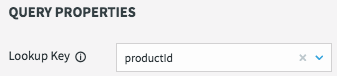 The lookup key for this cache is the primary key of the database table, or productId in this case.
All we need to do now is define how the cache obtains the data. This is done by setting the username, password, and connection URL information for the MySQL database, then selecting a table, or a query to run to access the data.
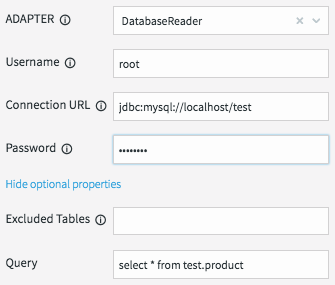
When the application is deployed, the cache will execute the query and load all the data returned by the query into the in-memory data grid; ready to be joined with our stream.
Loading the location information from a file requires similar steps. The file in question is a comma-delimited list of locations in the following form:
Location ID, City, State, Latitude, Longitude, Population
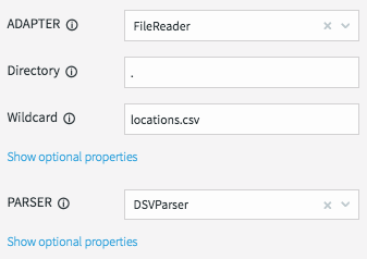
We will create a File Cache called “LocationInfo” to read and parse this file, and load it into memory assigning correct data types to each column.
The lookup key is the location id. ![]()
We will be reading data from the “locations.csv” file present in the product install directory “.” using the DSVParser. This parser handles all kinds of delimited files. The default is to read comma-delimited files (with optional header and quoted values), so we can keep the default properties.
As with the database cache, when the application is deployed, the cache will read the file and load all the data into the in-memory data grid ready to be joined with our stream.
Joining Streaming and Cache Data For Enrichment With SQL
The final step is to join the data in the caches with the real-time data coming from the MySQL CDC stream. This can be achieved by modifying the ExtractFields query we wrote earlier.
All we are doing here is adding the ProductInfo and LocationInfo caches into the FROM clause, using fields from the caches as part of the projection, and including joins on productId and locationId as part of the WHERE clause.
The result of this query is to continuously output enriched (denormalized) events for every CDC event that occurs for the PRODUCT_INV table. If the join was more complex – such that the ids could be null, or not match the cache entries – we could change to use a variety of join syntaxes, such as OUTER joins, on the data. We will cover this topic in a subsequent blog.
When the query is saved, the dataflow changes in the UI to show that the caches are now being used by the continuous query.
If we deploy and start the application, then preview the data on the stream prior to writing to Kafka we will see the fully-enriched records.
The data delivered to Kafka as JSON looks like this.
{
“locationId“:9,
“productId“:152,
“stock“:1277,
“prevStock“:1383,
“updateTime“:”2018-03-27T17:28:45.000-07:00”,
“description“:”Dorcy 230L ZX Series Flashlight”,
“price“:33.74,
“brand“:”Dorcy”,
“category“:”Industrial”,
“worn“:”Hands”,
“city“:”Dallas”,
“state“:”TX”,
“longitude“:-97.03,
“latitude“:32.9
}
As you can see, it is very straightforward to use the Striim platform to not only integrate streaming data sources using CDC with Apache Kafka, but also to leverage SQL-based stream processing and enrich the data-in-motion without slowing the data flow.
In the next tutorial, I will delve into delivering data in different formats to multiple targets, including cloud blob storage and Hadoop.