Striim TQL vs. KSQL: An Analysis of Streaming SQL Engines

Streaming Data Integration

Rajkumar Sen, Alok Pareek, Rohit Dubey

9 Minute Read

The following blog outlines some benchmarks on streaming SQL engines that we cited in our recent paper, Real-time ETL in Striim, at VLDB Rio de Janeiro in August 2018.

BIRTE ’18
Proceedings of the International Workshop on Real-Time Business Intelligence and Analytics
Article No. 3

In the past couple of years, Apache Kafka has proven itself as a fast, scalable, fault-tolerant messaging system, and has been chosen by many leading organizations as the standard for moving data around in a reliable way. Once data has landed into Kafka, enterprises want to derive value out of that data. This fueled the need to support a declarative way to access, manage and manipulate the data residing in Kafka. Striim introduced its streaming SQL engine, TQL (Tungsten Query Language), in 2014 for data engineers and business analysts to write SQL-style declarative queries over streaming data including data in Kafka topics. Recently, KSQL was announced as an open source, streaming SQL engine that enables real-time data processing against Apache Kafka.

In this blog post, we will attempt to do a competitive analysis of these streaming SQL engines – Striim’s TQL Engine vs. KSQL – based on two dimensions (a) Usability and (b) Performance. We will compare and contrast approaches taken by both the platforms and we will use two workloads to test the performance of both the engines:

Workload A: We use the ever popular data engineering benchmark TPCH and use a representative query (with modifications for streaming).
Workload B: We use a workload clickstream-analysis that is part of KSQL’s github page and use a query file that is also part of KSQL’s sample query set.

Usability

In this section, we will spend some time discussing how the two platforms differ in terms of basic constructs and capabilities. In every streaming compute/analytics platform, the following constructs are core to developing applications:

Streams: A stream is an unbounded sequence or series of data
Windows: A window is used to bound a stream by time or count
Continuous Queries: Continuously running SQL-like queries to filter, enrich, aggregate, join and transform the data.
Caches: A cache is set of historical or reference data to enrich streaming data
Tables: A table is a view of the events(rows) in a stream. Rows in a Table are mutable, which means that existing rows can be updated or deleted.

In addition to the above core constructs, because of the high volume and velocity of today’s streaming applications, all streaming platforms must be horizontally and vertically scalable. Also, because of the business nature of the data, all platforms must support Exactly Once Processing (E1P) semantics even for non-replayable sources.

In the following table, we will highlight some differences between Striim TQL and KSQL in terms of how core streaming compute constructs are defined and managed.

Construct	KSQL	TQL
Streams	No in-memory version. Always required a disk-based Kafka topic.	Both in-memory and persisted versions.
Windows	No attribute (column)-based time windows. Same window cannot be used in multiple queries.	Supports all types of windows. Same window can be used in multiple queries, amortizing memory cost.
Queries	No support for grouping on derived columns, limited aggregate support and no inner join	Supports all types of join, and aggregate queries.
Caches	Maintain external cache	In-house built cache with refresh
Tables	Has external dependency on RocksDB	In-house built EventTable

Performance Using Workload A

In this section, we will attempt to do a performance evaluation of the two platforms using a well-known benchmark in the data engineering space. We selected the TPCH benchmark, which is a very popular analytics benchmark amongst the data processing vendors, and modified the core nature of the queries from batching to streaming. The experiments were conducted in an EC machine of type i3xlarge.

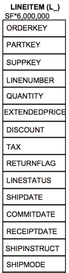
As KSQL does not support inner joins, we were very limited by what we could potentially run in KSQL since most of the queries in TPCH require inner join support. So, we limited ourselves to just one query that had some kind of filtering and aggregation. We generated data for Scale Factor 10 which led to a rowcount of 60M for the lineitem table. In order to make the workload streaming, we introduced timestamps (borrowed from Lorderdate from Orders table) in the rows so that we could apply windowing and aggregation on the data. Here is the schema for the lineitem table (prior to adding timestamps).

We then performed a set of experiments.

The first experiment is when the data comes in as raw files and being constantly fed to Striim TQL Engine. This experiment could not be repeated for KSQL since KSQL can only get data from Kafka topics.
The second experiment is when the data comes in as events in a Kafka topic. Striim TQL can directly read from Kafka topics (by using a construct called persisted streams that directly map to a Kafka topic).

We selected TPCH Q6 that has a filter and an aggregation.

SELECT
    sum(l_extendedprice * l_discount) as revenue
FROM
    lineitem
WHERE
    l_shipdate >= date '1994-01-01'
    AND l_shipdate < date '1994-01-01' + interval '1' year
    AND l_discount between 0.05 AND 0.07
    AND l_quantity < 24;

Since we had to convert the query to something that made sense in a streaming environment, we removed the predicates on l_shipdate and instead applied a 5 minute jumping (also commonly known as tumbling) window on the streaming data as it comes in while still retaining the predicates on l_discount, l_quantity and aggregate on l_extendedprice and l_discount. The original query gets converted to the following pseudo-queries

First create a stream S1 based on the stream of rows in the fact table lineitem
Filter out rows in S1 based on the predicates on l_discount and l_quantity
The filtered rows would keep forming 5 minute windows
- For each window, compute the aggregate and output to a result Kafka topic

KSQL

We inserted all the data in a Kafka topic line_10 and executed the following queries. Since KSQL did not support the original form of the query, we had to insert an arbitrary column ‘group_key’ (that had a single unique value) and use it for the grouping. The output of the final query also goes to a Kafka table named line_query6.

CREATE STREAM lineitem_raw_10 (shipDate varchar, orderKey bigint, discount Double , extendedPrice Double,  suppKey bigint, quantity bigint, returnflag varchar, partKey bigint, linestatus varchar, tax double , commitdate varchar, recieptdate varchar,shipmode varchar, linenumber bigint,shipinstruct varchar,orderdate varchar, group_key smallint) WITH (kafka_topic='line10', value_format='DELIMITED'); 

CREATE STREAM lineitem_10 AS 
Select STRINGTOTIMESTAMP(orderdate, 'yyyy-MM-dd HH:mm:ss') , orderkey, discount, suppKey, extendedPrice , quantity, group_key from lineitem_raw_10 where quantity<24 and   discount <0.07 and discount >0.05;

CREATE TABLE line_query6 AS Select  group_key, ,sum(extendedprice * (1-discount)) as revenue from lineitem_10  WINDOW TUMBLING (SIZE 5 MINUTES) GROUP BY group_key;

TQL

In Striim, there are several ways to enabling the same workload. Striim allows data to be directly read from files and also from Kafka topics thereby preventing a complete IO cycle.

In order to be compatible (testing wise) with KSQL, we loaded the data into a Kafka topic ‘LineItemDataStreamAll’ and modeled it as a persisted stream ‘LineItemDataStreamAll’. We wrote the following TQL queries, where the final query writes the results to a Kafka topic named LineDiscountStreamGrouped. Alternatively the first query LineItemFilter could also be done via an in-built adapter of Striim named KafkaReader.

CREATE CQ LineItemFilter
INSERT INTO LineItemDataStreamFiltered
select * from LineItemDataStreamAll l
WHERE l.discount >0.05 and l.discount <0.07 and l.quantity < 24
;

CREATE JUMPING  WINDOW LineWindow OVER LineItemDataFilterStream6 KEEP WITHIN 5 MINUTE ON LOrderDate;
;

CREATE TYPE ResultType (
   Group_key Integer,
  revenue Double
);
create stream LineDiscountStreamGrouped of ResultType
persist using KafkaProps;


CREATE OR REPLACE CQ LineItemDiscount
INSERT INTO LineDiscountStreamGrouped
Select
group_key, SUM(l.extendedPrice*(1- l.discount)) as revenue
 from LineWindow2Mins l
Group by group_key

Performance Numbers

We measured the execution time and average event throughput for both the platforms. We also tried a variant where we only performed the filter (more like an ETL case) and not the windowing and subsequent aggregation. The following are the total execution times and average event throughput for both the platforms. We used Striim 3.7.4 and KSQL 0.4 for the experiments.

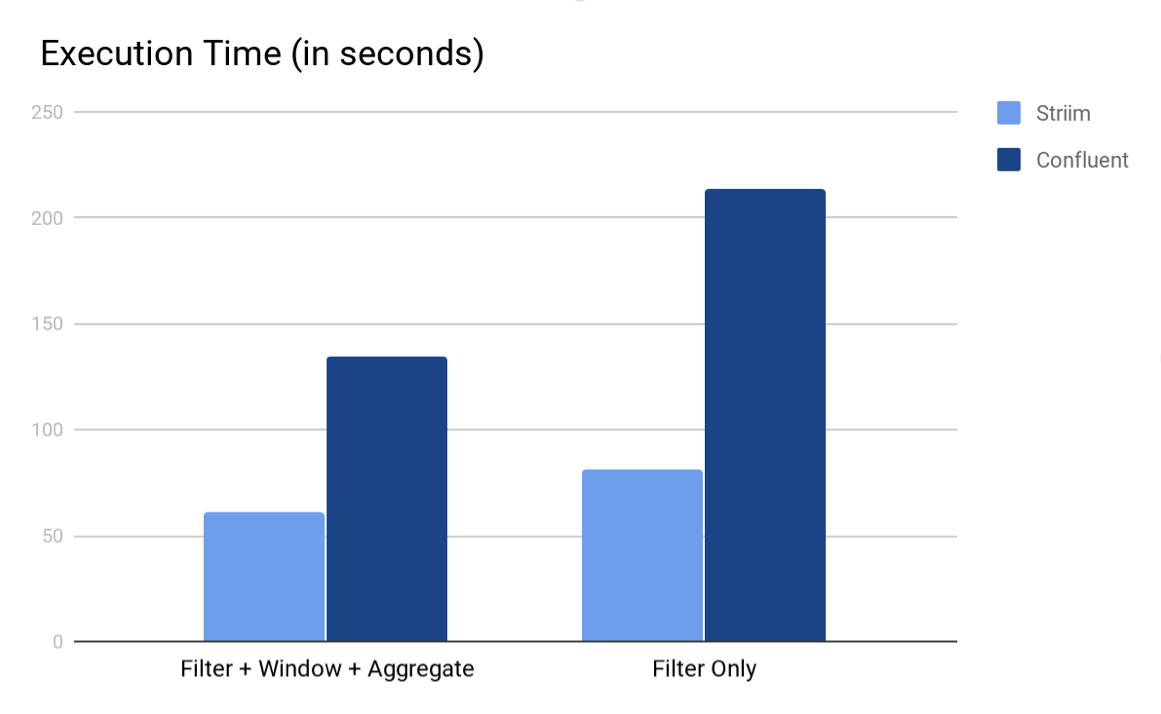
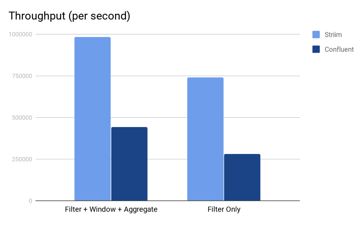
As we can see from both the charts, Striim’s TQL beat KSQL in both the scenarios. We believe that the main reason why Striim outperforms KSQL is because in Striim, the entire computation pipeline can be run in-memory whereas for KSQL, the output of every KSQL query is either a stream or a table which are backed by (disk-based) Kafka topics. Another interesting element is partitioning; in this experiment we could not partition the data because the aggregate query did not have any inherent grouping. Having said that, if there is partitioning in the storage and querying, Striim would also benefit from running computation tasks in parallel.

Another point to note is that KSQL is severely constrained on how many analytical query forms it can run since it still doesn’t support inner joins and aggregation like avg or count distinct without a grouping key. Till KSQL adds these core capabilities to the product, we really cannot compare performance of analytical queries across the two platforms.

Performance Using Workload B

As mentioned in the last section, KSQL is severely constrained on the types and forms of analytical query forms it can support and run, it was very hard to do an apples to apples comparison with Striim, since Striim TQL is very feature rich and can run many complex forms of streaming analytics queries. Therefore, in order to make a realistic comparison, we decided to pick a dataset and query from the KSQL github page and used to run the next set of experiments. The experiments were conducted in an EC machine of type i3xlarge.

The dataset that we picked up in the clickstream dataset that is available in the KSQL github page and we picked up the following sample query from one of their files clickstream-schema.sql. We ran the following queries that fall into the category of streaming data enrichment where the incoming streaming data is enriched with data that belongs to a another table or cache (one use case mentioned in this KSQL article).

KSQL Queries

CREATE STREAM clickstream (_time bigint,time varchar, ip varchar, request varchar, status int, userid int, bytes bigint, agent varchar) with (kafka_topic = 'clickstream', value_format = 'json');

CREATE TABLE WEB_USERS (user_id int, registered_At long, username varchar, first_name varchar, last_name varchar, city varchar, level varchar) with (key='user_id', kafka_topic = 'clickstream_users', value_format = 'json');

CREATE STREAM customer_clickstream WITH (PARTITIONS=2) as SELECT userid, u.first_name, u.last_name, u.level, time, ip, request, status, agent FROM clickstream c LEFT JOIN web_users u ON c.userid = u.user_id;

CREATE TABLE custClickStream as select * from customer_clickstream ;

We then used Striim to run a similar query where you read and write from Kafka. We used KafkaReader with JSON Parser to read into a typed stream. For “users” data set we loaded Striim’s refreshable cache component before performing the join. And the resulting stream is written back to Kafka as a new topic via the KafkaWriter. Striim TQL for the same is as follows:

CREATE STREAM clickStrm1 of clickStrmType;
CREATE SOURCE clickStreamSource USING KafkaReader (
 brokerAddress:'localhost:9092',
 Topic:'clickstream',
 startOffset:'0'
)
PARSE USING JSONParser (
 eventType:'admin.clickStrmType'
)
OUTPUT TO clickStrm1;

CREATE CQ customer_clickstreamCQ
INSERT INTO customer_clickstream1
select c.userid,u.first_name,u.last_name,u.level,c.time,c.ip,c.request,c.status,c.agent
From clickStrm1 c LEFT JOIN users_cache u
on c.userid = u.user_id ;

create Target writer using KafkaWriter VERSION '0.10.0' (
        brokerAddress:'localhost:9092',
        Topic:'StriimclkStrm'
)
format using JSONFormatter (
        EventsAsArrayOfJsonObjects:false,
        members:'userid,first_name,last_name,level,time,ip,request,status,agent'
)
INPUT FROM customer_clickstream1;

It is worthwhile to note here that even though we read and write to Kafka in this experiment, Striim is not limited to reading data from Kafka alone. Striim supports a much wider variety of input sources and output targets.

Performance Numbers

We measured the execution time and average event throughput for both the platforms for the following datasets

(a) DataSet1: 2 million rows in clickstream topic and 4 thousand rows in users topic.

(b) DataSet2: 4 million rows in clickstream topic and 8 thousand rows in users topic.

The data was generated using scripts provided by KSQL github page; both KSQL and Striim consumed data from the same Kafka topic named clickstream.

The following are the total execution times and average event throughput for both the platforms. We used Striim 3.7.4 and KSQL 0.4 (released December 2017) for the experiments.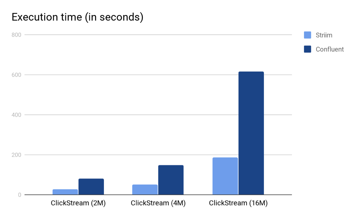
As we can see from both the charts, Striim’s TQL beat KSQL in both the scenarios by a multiple of 3. Again, we believe that the main reason why Striim outperforms KSQL is because in Striim, the entire computation pipeline can be run in-memory whereas for KSQL, the output of every KSQL query is either a stream or a table which are backed by (disk-based) Kafka topics. Also, since the input Kafka topic is partitioned, Striim was able to employ auto-parallelism and use multiple cores to read from Kafka, perform the query and write to the output Kafka topic.

Hardware

The experiments were all done using an EC2 machine of type i3xlarge. The hardware configuration is as follows

4 vCPUs each vCPU (Virtual CPU) is a hardware hyperthread on an Intel E5-2686 v4 (Broadwell) processor running at 2.3 GHz.
30.5 GB RAM
We used EBS-disk for storage.

Code

All the code that was used to run the experiments on streaming SQL engines is available in Striim’s github page in https://github.com/striim/KSQL-Striim.