Time series forecasting and anomaly detection
Striim now supports forecasting and anomaly detection on time-series data, using sophisticated machine learning models. These are implemented as built-in functions. Striim allows you to apply these models to your streaming data for data preprocessing and to analyze your streaming data for automated prediction, and anomaly detection.
Machine learning pipeline for prediction and anomaly detection
The following steps are involved in forecasting/anomaly detection:
Data processing: Before fitting data into sophisticated models, we recommend transforming and preprocessing the data. Striim supports a collection of data preprocessing methods including standardization and normalization to make training less sensitive to the scale of features, power transformation (like square root, log) to stabilize volatile data, and seasonality decomposition like Loess or STL decomposition to remove the seasonality in time-series data.
Automated prediction: Striim transforms time series regression to a standard regression problem with lagged variables (that is, autoregression), and then applies a regression model to it for prediction. This topic describes the random forest model.
Anomaly detection: Striim detects anomalies by comparing predicted values to actual values, flagging instances where the percentage error exceeds a statistically defined threshold. It assumes the percentage errors follow a normal distribution and sets the threshold based on this assumption.
Time series forecasting
This model allows you to forecast a future value based on previous ones with a random forest. Consider a time series consisting of N data points, represented as (ti, vi) for i = 1, 2, …, N, where ti denotes the timestamp and vi is the corresponding observed value.
Forecasting: The objective is to predict future values of the time series at upcoming timestamps tN+1, tN+2, and so on. These predictions are based on patterns learned from the existing data.
Anomaly Detection: When the actual value at a future timestamp (e.g., vN+1) becomes available, it can be compared with the predicted value. If the difference between the actual and predicted values exceeds a defined threshold, the data point is flagged as an anomaly.
Seasonality Decomposition: If the time series exhibits recurring seasonal patterns (e.g., temperature rises at noon each day), we can decompose the time series to isolate the seasonal component. The deseasonalized data can then be used as input to forecasting models such as Random Forest.
Using Foreseer in Flow Designer
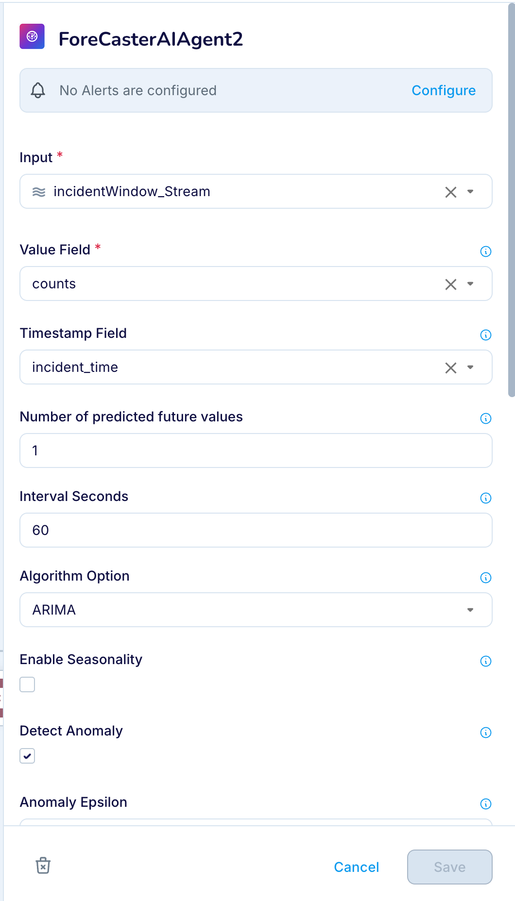
You can configure time series forecasting and anomaly detection in the Flow Designer using the Foreseer AI Agent. This allows you to analyze streaming data without writing TQL manually.
To use Foreseer:
In Flow Designer, open the canvas for your application flow.
From the AI Agent menu, drag a Foreseer component onto the canvas.
Connect the Foreseer node to an input stream or preprocessing logic (e.g., via a sliding window).
Configure the Foreseer node’s options, such as number of predicted future values and timestamp interval, anomaly threshold, and seasonal parameters, through the node properties panel.
Connect Foreseer’s output to downstream sinks or dashboards for further analysis or alerting.
Using Foreseer from Flow Designer simplifies integration and lets you visually manage anomaly detection and forecasting logic in real-time data flows.
Viewing and interpreting anomaly detection results
After running your real-time forecasting and anomaly detection pipeline, you can visualize the results using a time series chart. This visualization helps you compare actual values to predicted values and highlights anomalies based on deviation thresholds.
The chart typically includes:
Actual values: the raw observed data points over time.
Predicted values: values forecasted by the Foreseer AI agent using historical trends and time series models such as statistical or machine learning algorithms.
Anomalies: points where the actual value significantly diverges from the prediction, exceeding a statistical error threshold.
The following example visualization illustrates how anomalies (red markers) are detected where the actual time series deviates beyond the expected prediction range:
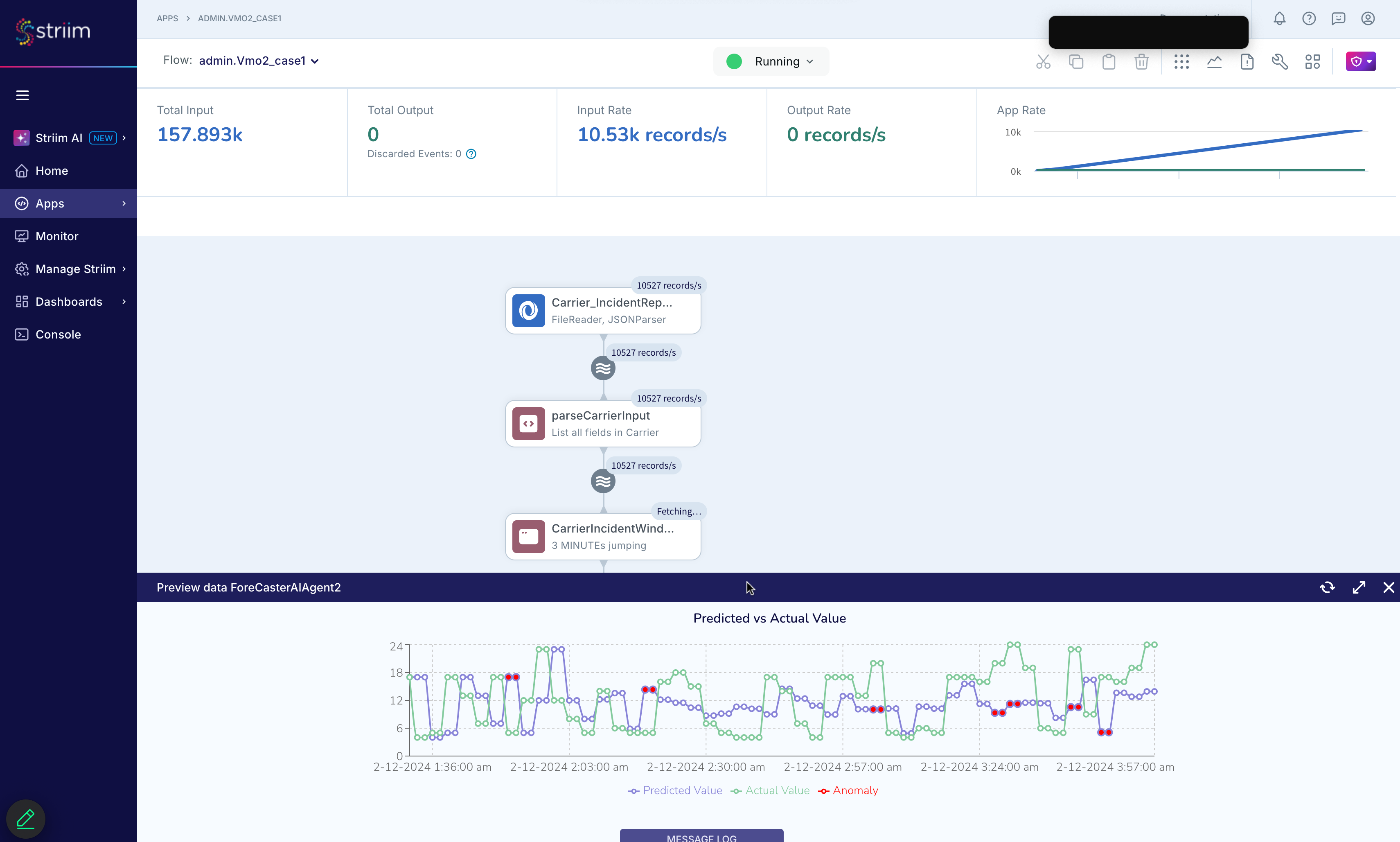
This graphical output helps validate the accuracy of the model and supports use cases such as system monitoring, fraud detection, or infrastructure anomaly tracking.
Forecast Function
Syntax
The forecast function is used within a continuous query (CQ) and follows the format:
      SELECT forecast(<Double field name>, <DateTime field name>, <int>, [ <JsonNode> ])
      FROM <stream name>
Examples:
      SELECT forecast(V, TS, 60) FROM S;
      SELECT forecast(V, null, 1) FROM S;
Vmust be of typeDouble. If it is another numeric type, useto_double(V).TSmust be of typeDateTime. Usenullif no timestamp is available.The third argument is the interval in seconds between data points (e.g.,
60means one point per minute).The fourth argument is optional and can be a configuration object in
JsonNodeformat.
Semantics
The forecast function must be used after a sliding window is applied in a continuous query. The sliding window groups recent time series data into a windowed batch, and forecast operates on that batch to generate predictions for future values.
In a stream S, field TS represents the timestamps of the time series data, and V contains the corresponding values. If the timestamp interval is 60 seconds, then each data point is evenly spaced in time such that:
ti+1 = ti + 60 seconds
The forecast function uses the provided values to predict future points based on historical patterns. When a timestamp field (TS) is not available, you can set the timestamp argument to null. In this case, the forecast assumes that the values in V are evenly spaced, and the interval is defined by the third argument (e.g., 1 for unit spacing).
The return type of the forecast function is ForecastResult, which is described in the next section.
Pipeline
The forecast continuous query (CQ) should operate on data produced by a jumping window. Using a jumping window avoids duplicate data points in the forecast input. The size of the jumping window determines how much recent data is used for prediction.
For example, if the jumping window covers a 3-minute interval, the forecast function will use data from the most recent 3 minutes. The overall data pipeline can be represented as:
Stream S → Jumping Window W → Forecast CQ → Output S
Options
You can pass hyperparameters to the forecast function using a JsonNode. The supported options are listed below:
numStepsToPredict(integer): Number of future steps to predict. Default is1.retrainFrequency(integer): How often to retrain the ML model. Default is10(the model will be retrained only after 10 new data points).detectAnomaly(boolean): Whether to enable anomaly detection. Default istrue.anomalyEpsilon(double between 0 and 1): Sensitivity of anomaly detection. Default is0.05. Higher values flag more points as anomalies.anomalyLength: Specifies the minimum number of consecutive anomalies required before an alert is triggered. This helps reduce false positives by ensuring that only sustained anomalies generate alerts. The default value is1.anomalyStart(integer): Start detecting anomalies after N data points. Default is30. RequiresdetectAnomaly=true.enableSeasonality(boolean): Decompose seasonality before prediction. Default isfalse.seasonalLength(integer): Length of the seasonal cycle. For example, set to24for hourly data with daily seasonality. Default is1440.missingValueOption(string): Strategy for handling missing values. Options:"ignore"(default) or"zero".algorithmOption(string): Forecasting algorithm to use. Options:"randomForest"or"arima". Default is"arima".
Example CQ with custom options:
      SELECT forecast(opNum, opTime, 60, makeJson(
        "{\"detectAnomaly\": false, \"numStepsToPredict\": 20}"
      )) AS val,
      val.currentTimestamp AS currentOpTime,
      val.actualValue AS actual,
      val.predictedValue AS predict,
      val.adjustedSymmetricPercentageError AS aspe,
      val.percentageErrorBound AS errorBound,
      val.isAnomaly AS isAnomaly,
      val.nextTimestamp AS nextOpTime,
      val.nextPredictedValue AS nextPredicted
      FROM forecast_win;
GroupBy
You can use the GROUP BY clause to apply forecasting to grouped subsets of data. For example, suppose a stream S contains three fields: timestamp, operationNum, and tableName. The stream records the number of operations on different tables every minute.
To forecast future operation counts for each table individually:
      SELECT tableName, forecast(operationNum, operationTime, 60) AS val,
      val.currentTimestamp AS currentOpTime,
      val.actualValue AS actual,
      val.predictedValue AS predict,
      val.adjustedSymmetricPercentageError AS aspe,
      val.percentageErrorBound AS errorBound,
      val.isAnomaly AS isAnomaly,
      val.nextTimestamp AS nextOpTime,
      val.nextPredictedValue AS nextPredicted
      FROM forecast_win
      GROUP BY tableName;
Note: The GROUP BY tableName clause is required to apply the forecast per table.
Missing Value Handling
The forecast function supports two methods for handling missing values in time series data: "ignore" and "zero". This is controlled by the missingValueOption parameter.
Let’s consider a time series with timestamps and values:
    t1 = 14:00 → v1
    t2 = 14:01 → v2
    t3 = 14:03 → v3
The expected interval is 1 minute, so the timestamp 14:02 is considered missing.
"ignore"(default): The missing timestamp is ignored. Only existing values (v1,v2,v3) are used for forecasting."zero": Missing values are filled with0. In this case, the series becomesv1,v2,0,v3.
To detect missing data points, the forecast engine uses the first timestamp t0 and the specified interval s. The expected timestamp for the k-th data point must fall within the interval:
[t0 + (k-1) * s, t0 + k * s]
If a data point does not fall within this expected interval, it is treated as missing.
ForecastResult type
The forecast function returns a value of type ForecastResult, which includes the following fields:
Field | Type | Description |
|---|---|---|
currentTimestamp | DateTime | The current timestamp for the data point. |
actualValue | Double | The actual value for the current timestamp. |
predictedValue | Double | The predicted value for the current timestamp. |
adjustedSymmetricPercentageError | Double | The percentage error between the actual and predicted values. After we scale actual and predicted values using By default, the actual and predicted are scaled to 100 to 200. |
percentageErrorBound | Double | A dynamic threshold for the percentage error. We identify an anomaly, if the |
isAnomaly | Boolean | True, if it is detected as an anomaly. |
nextTimestamp | DateTime | The nextTimestamp is determined by the currentTimestamp plus an interval. |
nextPredictedValue | Double | A predicted value for the next timestamp. |
predictedValueList | List<Double> | The predicted values for the next few timestamps. You can specify how many steps you want to look ahead in the option. |
timestampList | List<Double> | The next few timestamps corresponding to the predictedValueList. If the current timestamp is null, the list will be an empty list. |
Example TQL application: real-time forecasting and anomaly detection
This example TQL application implements a real-time forecasting and anomaly detection pipeline for incident report data streamed from JSON log files. The application reads incident data, aggregates it in 3-minute windows, and applies a forecasting model to detect anomalies in incident rates. Alerts for anomalous activity are published to Slack, and forecasting results are stored in a WActionStore.
CREATE OR REPLACE APPLICATION Example_case1;

CREATE OR REPLACE SOURCE IncidentReports USING Global.FileReader (
  directory: '/Users/user/Documents/CSVData/incident_files_generated/',
  adapterName: 'FileReader',
  rolloverstyle: 'Default',
  wildcard: '*.log',
  blocksize: 64,
  skipbom: true,
  includesubdirectories: false,
  positionbyeof: false )
PARSE USING Global.JSONParser (
  fieldName: '',
  handler: 'com.webaction.proc.JSONParser_1_0',
  parserName: 'JSONParser' )
OUTPUT TO IncidentReports_stream;

CREATE OR REPLACE TYPE IncidentWStype (
 currentOpTime org.joda.time.DateTime,
 actual java.lang.Double,
 predicted java.lang.Double,
 isAnomaly java.lang.Boolean);

CREATE OR REPLACE TYPE IncidentOutput_type (
 val com.webaction.analytics.forecast.ForecastResult,
 currentOpTime org.joda.time.DateTime,
 actual java.lang.Double,
 predicted java.lang.Double,
 aspe java.lang.Double,
 errorBound java.lang.Double,
 isAnomaly java.lang.Boolean,
 nextOpTime org.joda.time.DateTime,
 nextPredicted java.lang.Double);

CREATE OR REPLACE CQ parseInput
INSERT INTO IncidentReports
SELECT TO_DATE(TO_STRING(TO_DATE(a.data.get('incident_data').get('incident_time').textValue()),
"yyyy-MM-dd HH:mm:00")) as incident_time, a.data.get('incident_data').get('cause') as cause
FROM IncidentReports_stream a;

CREATE OR REPLACE WACTIONSTORE IncidentWS CONTEXT OF IncidentWStype EVENT TYPES
( IncidentWStype KEY(currentOpTime) );

CREATE OR REPLACE STREAM IncidentForecastResult OF IncidentOutput_type;

CREATE OR REPLACE JUMPING WINDOW IncidentWindow OVER IncidentReports
KEEP WITHIN 3 MINUTE ON incident_time;

CREATE OR REPLACE STREAM IncidentAlertStream of Global.AlertEvent;


CREATE OR REPLACE CQ IncidentAgg
INSERT INTO incidentWindow_Stream
SELECT count(*) as count, first(incident_time) as incident_time
FROM IncidentWindow;;

CREATE OR REPLACE CQ Incident_Analyser
INSERT INTO IncidentForecastResult
SELECT forecast(to_double(e.count),e.incident_time, 60, makeJson("{\"anomalyEpsilon\": 0.20}")) as val,
val.currentTimestamp as currentOpTime,
val.actualValue as actual,
val.predictedValue as predicted,
val.adjustedSymmetricPercentageError as aspe,
val.percentageErrorBound as errorBound,
val.isAnomaly as isAnomaly,
val.nextTimestamp as nextOpTime,
val.nextPredictedValue as nextPredicted
FROM incidentWindow_Stream e;

CREATE OR REPLACE CQ incidentAnomalyAlertGenerator
INSERT INTO IncidentAlertStream
SELECT "Incidents", "Actual: " + TO_STRING(e.actual) + "; Predicted: " + TO_STRING(e.predicted),
"error", "notify", "We are seeing abnormal Incident rate."
FROM IncidentForecastResult e;;

CREATE OR REPLACE TARGET SlackTarget USING Global.SlackAlertAdapter (
  adapterName: 'SlackAlertAdapter',
  OauthToken: 'OauthToken',
  refreshtokenrenewal: false,
  OauthToken_encrypted: 'true',
  ChannelName: 'slack-test' )
INPUT FROM IncidentAlertStream;

CREATE OR REPLACE CQ IncidentWSWriter
INSERT INTO IncidentWS
SELECT currentOpTime, actual, predicted, isAnomaly
FROM IncidentForecastResult;

END APPLICATION Example_case1;